Chapter 2: Foundation Models / Large Language Models¶

Download this page as PDF

PDFs mapped: AI_Engineering_WS20252026_Ch2.1-2.3.pdf, Ch2.4-2.5part1.pdf, Ch2.5part2.pdf, Ch2.5part3-Ch2.7.pdf, Ch2.8-Ch2.10part1.pdf, Ch2.10part2-Ch2.12part1.pdf, Ch2.12part2-Ch4part1.pdf (the LLM portion) Code mapped: 1-1-llms.ipynb (and the HTML render 1-1-llms.html)

This is the largest and most exam-critical chapter of the course (TU Braunschweig, AI Engineering, WS 25/26). Every later chapter — Prompting (Ch. 3), RAG (Ch. 4), Agents (Ch. 5), Fine-tuning (Ch. 6) — is justified by mechanics introduced here.

Exam Profile (read this first)¶

Property	Value
Duration / points	120 minutes, 50 points, in English
Allowed aids	non-programmable calculator
Fundamentals questions	multiple choice, exactly one correct option ("Which statement best describes…")
Analysis questions	"Explain why…", 3 points — answer as cause → mechanism → consequence
Application questions	mini-case, 5 points — name the technique, give a justification, state a trade-off
Instructions on the sheet	"Use the technical terms from the lecture. Do not use abbreviations."
Numeric answers	round to 2 decimal places

The released sample exam contained a multiple-choice question on cosine similarity of embeddings (Section 2.4) and a free-text question on deduplication of training data (Section 2.1). Both sections below are therefore treated with extra depth.

বাংলা ব্যাখ্যা: পরীক্ষায় ফর্মুলা মুখস্থ থাকা যথেষ্ট নয় — ছোট সংখ্যা দিয়ে হাতে হিসাব করতে পারতে হবে (ক্যালকুলেটর non-programmable)। প্রতিটি "Explain why" উত্তরে কারণ → কীভাবে ঘটে → ফলাফল, এই তিন ধাপ লিখলে পুরো নম্বর পাওয়া যায়। আর মনে রেখো: সংক্ষিপ্ত রূপ (abbreviation) লেখা যাবে না — যেমন "RLHF" নয়, লিখতে হবে "Reinforcement Learning from Human Feedback"।

Chapter Roadmap¶

This chapter explains how a large language model is built end-to-end:

Where the data comes from (2.1)
How text becomes numbers: Tokenization (2.2) → Input/Output Pipeline (2.3) → Embeddings (2.4)
How the transformer processes those numbers (2.5)
The architectural variants used in 2024/25 models (2.6)
How the model chooses the next token: decoding and sampling (2.7)
How the model is pretrained (2.8) and how it adapts at runtime via in-context learning (2.9)
How it is aligned to be helpful and safe: supervised fine-tuning, reinforcement learning from human feedback, direct preference optimization (2.10)
Scaling laws that govern model/data/compute trade-offs (2.11)
How we evaluate the result (2.12)

Story for intuition. Imagine teaching a child a language with no grammar book — only millions of stories. After enough reading, the child predicts words, then sentences, then jokes. It does not "understand" the world, but its next-word predictions become eerily good. An LLM is that child, scaled to "all of Wikipedia, Reddit, GitHub, and arXiv". To make that work as an engineering system you need: words → numbers (tokenization, embeddings), numbers → context-aware numbers (attention), numbers → next-word probabilities (output projection + softmax), a way to pick one word (sampling), and a way to train (gradient descent, then alignment).

বাংলা ব্যাখ্যা: পুরো অধ্যায়টা আসলে একটাই গল্প — কাঁচা টেক্সট থেকে শুরু করে একটা চ্যাট-সহকারী পর্যন্ত পুরো পাইপলাইন। ডেটা → টোকেন → ভেক্টর → ট্রান্সফরমার → স্যাম্পলিং → প্রিট্রেইনিং → অ্যালাইনমেন্ট → মূল্যায়ন। পরীক্ষায় "কেন" ধরনের যে-কোনো প্রশ্নের উত্তর প্রায় সবসময় এই চেইনের কোনো একটা ধাপে লুকিয়ে আছে।

Glossary of Key Terms¶

Term	Meaning	বাংলা	Example
Token	smallest unit of text the model reads	মডেল যা পড়ে তার ক্ষুদ্রতম একক	"playing" → ["play", "ing"]
Vocabulary	the fixed set of all tokens the model knows	মডেলের শব্দভাণ্ডার (নির্দিষ্ট তালিকা)	size 32k (LLaMA-2) to 128k+ (LLaMA-3)
Byte-Pair Encoding (BPE)	greedy merge algorithm that builds a sub-word vocabulary	সবচেয়ে ঘনঘন আসা জোড়া বারবার জোড়া লাগানো	merge ("e","s") → "es"
Out-of-vocabulary (OOV)	input that no vocabulary entry covers	শব্দভাণ্ডারে নেই এমন ইনপুট	byte-level BPE never has OOV
Embedding	dense vector representation of a token	টোকেনের ভেক্টর-রূপ (অর্থের আঙুলের ছাপ)	a 4096-dimensional vector
Embedding matrix	lookup table of all token vectors, $E \in \mathbb{R}^{V \times d}$	সব টোকেনের ভেক্টরের টেবিল	row = one token's vector
Cosine similarity	angle-based similarity of two vectors	দুই ভেক্টরের কোণ-ভিত্তিক মিল	$\cos\theta = u \cdot v /(\lVert u\rVert\,\lVert v\rVert)$
Euclidean distance	straight-line distance between vectors	দুই বিন্দুর সরল দূরত্ব	$\lVert u - v \rVert_2$
Query / Key / Value	the three projections used by attention	প্রশ্ন / সূচক / বিষয়বস্তু — অ্যাটেনশনের তিন ভূমিকা	$Q = XW_Q$, $K = XW_K$, $V = XW_V$
Self-attention	each token attends to (mixes information from) other tokens of the same sequence	একই বাক্যের টোকেনরা একে-অপরের তথ্য মেশায়	scaled dot-product attention
Causal mask	hides future positions in decoder-only models	ভবিষ্যতের টোকেন লুকিয়ে রাখা	upper triangle set to $-\infty$
Multi-Head Attention (MHA)	several attention heads run in parallel	একসাথে অনেকগুলো অ্যাটেনশন-মাথা	h = 32 heads in LLaMA-7B
Grouped-Query Attention (GQA)	several query heads share one key/value head	কয়েকটা Q-মাথা একটাই K/V-মাথা ভাগ করে	LLaMA-3 uses 8 KV heads
Multi-Query Attention (MQA)	all query heads share a single key/value head	সব Q-মাথার জন্য একটাই K/V	extreme KV-cache saving
KV cache	stored keys/values of past tokens during generation	আগের টোকেনের K,V জমিয়ে রাখা	makes generation O(n) per token
Feed-forward network (FFN)	per-position multilayer perceptron inside a block	প্রতিটি অবস্থানে আলাদা ছোট নিউরাল নেট	expand 4×, then project back
SwiGLU	gated activation used in modern FFNs	আধুনিক FFN-এর গেটযুক্ত অ্যাক্টিভেশন	used in LLaMA, PaLM
LayerNorm / RMSNorm	normalization of activations for stable training	অ্যাক্টিভেশনের স্কেল ঠিক রাখা	RMSNorm drops mean-centering
Residual connection	skip connection around each sub-layer	শর্টকাট পথ: ইনপুট সরাসরি আউটপুটে যোগ	$y = x + \mathrm{Sublayer}(x)$
Positional encoding	injects token-order information	টোকেনের ক্রম/অবস্থান জানানো	sinusoidal, learned, RoPE
Rotary Position Embedding (RoPE)	encodes position by rotating query/key pairs	ভেক্টর ঘুরিয়ে অবস্থান বোঝানো	rotation angle ∝ position
Weight tying	input embedding matrix reused as output projection	একই ম্যাট্রিক্স ঢোকা ও বেরোনো দুই জায়গায়	saves $V \cdot d$ parameters
Logits	raw, unnormalized scores before softmax	softmax-এর আগের কাঁচা স্কোর	one number per vocabulary entry
Greedy decoding	always pick the highest-probability token	সবসময় সর্বোচ্চ সম্ভাবনার টোকেন	deterministic, can be repetitive
Temperature	rescales logits before softmax; controls randomness	আউটপুটের বৈচিত্র্যের নিয়ন্ত্রক	T < 1 sharper, T > 1 flatter
Top-k sampling	sample only among the k most probable tokens	সেরা k-টা থেকে বাছাই	k = 50 typical
Top-p (nucleus) sampling	sample among the smallest set with cumulative probability ≥ p	জমা সম্ভাবনা p ছোঁয়া পর্যন্ত টোকেন রাখা	p = 0.90 typical
Pretraining	self-supervised next-token training on web-scale data	বিশাল ডেটায় প্রাথমিক প্রশিক্ষণ	LLaMA-3: ~15 T tokens
Teacher forcing	training on all positions in parallel with true prefixes	আসল টেক্সট দিয়ে সব অবস্থানে একসাথে শেখানো	enables parallel training
Gradient accumulation	sum gradients over micro-batches before one optimizer step	ছোট ব্যাচ জমিয়ে বড় ব্যাচের প্রভাব	simulates large batch on small GPU
Mixed precision	compute in FP16/BF16, keep FP32 master weights	কম-বিট গণনা, বেশি-বিট সংরক্ষণ	halves memory, doubles speed
In-context learning	task adaptation via prompt examples, no weight update	প্রম্পটে উদাহরণ দেখিয়ে শেখানো	few-shot prompting
Supervised fine-tuning (SFT)	training on (instruction, ideal answer) pairs	আদর্শ উত্তর দেখিয়ে শোধন	InstructGPT step 1
Reward model	network scoring how much humans would prefer an answer	উত্তরের "মানুষ-পছন্দ" স্কোরার	trained with Bradley–Terry loss
Reinforcement Learning from Human Feedback (RLHF)	optimize the policy against the reward model with a KL leash	মানুষের পছন্দ অনুযায়ী RL	InstructGPT steps 2–3
Proximal Policy Optimization (PPO)	the clipped-ratio RL algorithm used in RLHF	RLHF-এর ভেতরের RL অ্যালগরিদম	clips policy ratio to 1 ± ε
Direct Preference Optimization (DPO)	closed-form supervised loss on preference pairs	reward model ছাড়াই পছন্দ-শেখা	no reward model, no RL loop
Scaling law	predictable loss decrease with more parameters/data/compute	বড় মডেল + বেশি ডেটা = নিয়মমাফিক কম লস	Chinchilla: D ≈ 20 N
Perplexity	exponentiated cross-entropy; "effective branching factor"	মডেল গড়ে কতগুলো অপশনে দ্বিধায়	lower is better
Benchmark	standardized evaluation set	মান-পরীক্ষার প্রশ্নব্যাংক	MMLU, HumanEval, GSM-8K
Contamination	test data leaked into training data	পরীক্ষার প্রশ্ন আগে থেকেই ট্রেনিং-ডেটায়	inflates benchmark scores

বাংলা ব্যাখ্যা: এই টেবিলটা পরীক্ষার আগের রাতে এক নজরে দেখার জন্য। মনে রাখার কৌশল: টোকেনাইজেশন = "টেক্সট কাটা", এমবেডিং = "অর্থের ভেক্টর", অ্যাটেনশন = "কে কার দিকে তাকাবে", স্যাম্পলিং = "পরের শব্দ বাছাই", অ্যালাইনমেন্ট = "ভদ্রতা শেখানো", স্কেলিং ল = "কত বড় বানাবো", ইভ্যালুয়েশন = "কতটা ভালো হলো"।

2.1 — Training Data¶

What the lecture says¶

Model parameters encode statistical regularities of the training corpus: grammar, world knowledge, style, reasoning patterns, pragmatics, task templates.
Performance collapses outside well-represented regions: "garbage in, garbage out."
Bias: training data inherits the internet's biases (gender, race, language, ideology). Bias is a data-level phenomenon — no architectural trick removes it.
Language bias: English is massively over-represented. Rule of thumb from the lecture: no Thai data → no Thai capability.
Curated open datasets: Common Crawl (raw web), The Pile, RedPajama, RefinedWeb, FineWeb / FineWeb-Edu (HuggingFace's filtered web corpora).
FineWeb pipeline: URL filtering → language identification → quality classification → deduplication → tokenization.
Scale references: GPT-3 ≈ 300 B tokens (mostly English); LLaMA-3.1 ≈ 15 T tokens (multilingual).

বাংলা ব্যাখ্যা: মডেল হলো "যা খায়, তাই" — ট্রেনিং ডেটাই তার জ্ঞান, ভাষা, এমনকি পক্ষপাতও ঠিক করে দেয়। ইংরেজি ডেটা বেশি বলে মডেল ইংরেজিতে ভালো; বাংলা বা থাই ডেটা কম বলে সেসব ভাষায় দুর্বল। ডেটার মান খারাপ হলে মডেলও খারাপ — architecture যত সুন্দরই হোক।

Deduplication (extra depth — appeared as free text in the sample exam)¶

What it is. Removing repeated content from the training corpus, at two granularities:

Exact deduplication — identical documents/lines are detected by hashing (e.g., MD5/SHA of normalized text) and all but one copy removed.
Near (fuzzy) deduplication — almost-identical documents (boilerplate, mirrored pages, license texts) are detected with MinHash signatures + locality-sensitive hashing over n-gram shingles; documents above a Jaccard-similarity threshold are collapsed.

Why it matters — the four-part exam answer (cause → mechanism → consequence):

Prevents memorization instead of generalization. A document seen 100 times receives 100× the gradient weight, so the model memorizes it verbatim instead of learning general patterns. Consequence: wasted capacity, verbatim regurgitation, privacy risk.
Stops implicit over-weighting of the duplicated distribution. Duplicates silently shift the effective data distribution toward whatever happens to be mirrored often (spam, SEO pages, license boilerplate) — equivalent to training extra epochs on the worst part of the web.
Improves compute efficiency. Every duplicated token costs the same FLOPs (Section 2.8: cost ≈ 6ND) but adds almost no new information; deduplication buys more unique tokens for the same compute budget.
Reduces benchmark contamination. Test sets circulate on the web; deduplication (against eval sets too) reduces the chance the model has literally seen the exam (Section 2.12).

Trade-off to mention in an application question: aggressive near-deduplication can delete legitimately frequent text (popular quotations, code idioms) and is computationally expensive at web scale (hence approximate methods like MinHash rather than exact pairwise comparison).

বাংলা ব্যাখ্যা: ডুপ্লিকেট ডেটা মানে একই পৃষ্ঠা মডেল বারবার পড়ছে — ফলে সে ওই টেক্সট মুখস্থ করে ফেলে, নতুন কিছু শেখে না, আর কম্পিউট নষ্ট হয়। তাছাড়া বেঞ্চমার্কের প্রশ্ন ওয়েবে ছড়িয়ে থাকে — ডিডুপ্লিকেশন না করলে মডেল "আগে দেখা প্রশ্নে" ভালো করে, যা আসল সক্ষমতা নয়। exact dedup হয় হ্যাশ দিয়ে, near-dedup হয় MinHash দিয়ে।

Code example — toy quality filter (FineWeb-style)¶

docs = [
    "The quick brown fox jumps over the lazy dog.",
    "Hi.",
    "The quick brown fox jumps over the lazy dog.",   # exact duplicate
    "x x x x",
    "Bonjour le monde.",                              # non-English
    "Climate change is a global challenge requiring policy and innovation."
]
seen = set()
filtered = []
for d in docs:
    if len(d.split()) < 5:        continue   # length / quality filter
    if d in seen:                 continue   # exact deduplication (hash set)
    if not d.isascii():           continue   # crude language filter
    seen.add(d)
    filtered.append(d)
print(filtered)   # 2 documents survive

The surviving 2 documents mirror what a real pipeline does: length/quality filter, exact deduplication via a hash set, language identification.

Common mistakes¶

"More data is always better." — false if quality is bad; FineWeb-Edu (smaller, classifier-filtered) beats raw Common Crawl.
Forgetting that data bias compounds through later alignment stages: the reward model is also trained by humans on top of a biased base.

2.2 — Tokenization¶

What the lecture says¶

LLMs only consume integer IDs; tokenization is the bridge from raw text to integer sequences, detokenization the inverse map.
Word-level tokenization: huge vocabulary, out-of-vocabulary problem for unseen words.
Character-level: tiny vocabulary but very long sequences (attention cost grows quadratically in length, Section 2.5).
Sub-word (BPE) is the compromise. Modern LLMs use byte-level BPE on raw UTF-8 bytes — every string is representable, so out-of-vocabulary never occurs.
Vocabulary sizes: ≈ 32k (LLaMA-2), ≈ 128k (LLaMA-3), ≈ 200k (GPT-4-class).
Special tokens: begin/end-of-sequence, padding, chat-role markers (e.g., <|im_start|>).
API cost is per token — tokenizer efficiency directly affects money. Rule of thumb: 1 token ≈ 0.75 English words (fewer for morphologically rich languages).

বাংলা ব্যাখ্যা: মডেল আসলে অক্ষর বা শব্দ চেনে না — চেনে শুধু সংখ্যা। টোকেনাইজার হলো অনুবাদক: টেক্সট → সংখ্যার তালিকা। শব্দ-স্তরে ভোকাব বিশাল হয়ে যায়, অক্ষর-স্তরে বাক্য অসম্ভব লম্বা হয়; তাই মাঝামাঝি সমাধান — ঘনঘন আসা অক্ষর-জোড়া জোড়া লাগিয়ে "সাব-ওয়ার্ড" বানানো। এটাই BPE।

BPE training algorithm¶

input  : corpus words split into characters, with an end-of-word marker </w>
output : ordered list of merge rules + final vocabulary

vocab <- set of characters
repeat until |vocab| reaches target size:
    count frequency of every adjacent symbol pair across the corpus
    best_pair <- the most frequent pair (ties: first encountered)
    merge best_pair into one new symbol everywhere; add it to vocab

At encoding time, the learned merges are replayed in order on new text.

Worked example — full BPE merge sequence on a toy corpus¶

Corpus (word : frequency): low:5, lower:2, newest:6, widest:3. Initial segmentation (with end-of-word marker </w>):

l o w </w>        x5
l o w e r </w>    x2
n e w e s t </w>  x6
w i d e s t </w>  x3

Step 0 — count all adjacent pairs:

Pair	Count	Pair	Count
(e, s)	6 + 3 = 9	(n, e)	6
(s, t)	6 + 3 = 9	(e, w)	6
(w, e)	2 + 6 = 8	(w, i)	3
(l, o)	5 + 2 = 7	(i, d)	3
(o, w)	5 + 2 = 7	(d, e)	3
(t, `</w>`)	9	(e, r)	2

Merge sequence (ties broken by first appearance):

#	Merge	Count	New symbol	Corpus state after merge
1	(e, s)	9	`es`	`n e w es t </w>` ×6, `w i d es t </w>` ×3
2	(es, t)	9	`est`	`n e w est </w>` ×6, `w i d est </w>` ×3
3	(est, `</w>`)	9	`est</w>`	`n e w est</w>` ×6, `w i d est</w>` ×3
4	(l, o)	7	`lo`	`lo w </w>` ×5, `lo w e r </w>` ×2
5	(lo, w)	7	`low`	`low </w>` ×5, `low e r </w>` ×2

Vocabulary after 5 merges: characters ∪ { es, est, est</w>, lo, low }.

Resulting tokenizations: "lowest" → [low, est</w>] (2 tokens, even though "lowest" never appeared in the corpus!); "low" → [low, </w>]; "newest" → [n, e, w, est</w>] until later merges create ne, new.

Why "lowering" still needs several tokens: no merge ever produced er or ing-like units from this tiny corpus, so rare suffixes stay as characters — frequent strings get short codes, rare strings get long codes (a compression view of BPE).

বাংলা ব্যাখ্যা: BPE-র মূল আইডিয়া: যেটা সবচেয়ে বেশি বার পাশাপাশি আসে, সেটাকে এক টোকেন বানাও — অনেকটা কম্প্রেশনের মতো। লক্ষ করো, "lowest" শব্দটা কর্পাসে ছিলই না, তবু low + est দিয়ে মাত্র ২ টোকেনে লেখা গেল — এটাই sub-word টোকেনাইজেশনের শক্তি: অদেখা শব্দও চেনা টুকরো দিয়ে গড়া যায়। পরীক্ষায় pair-count টেবিল বানিয়ে ধাপে ধাপে merge দেখাতে হবে।

Code example — BPE from scratch¶

from collections import Counter

def get_pairs(words):
    pairs = Counter()
    for w, freq in words.items():
        symbols = w.split()
        for a, b in zip(symbols, symbols[1:]):
            pairs[(a, b)] += freq
    return pairs

def merge(words, pair):
    a, b = pair
    return {w.replace(f"{a} {b}", f"{a}{b}"): f for w, f in words.items()}

words = {"l o w </w>": 5, "l o w e r </w>": 2,
         "n e w e s t </w>": 6, "w i d e s t </w>": 3}
for step in range(5):
    best = get_pairs(words).most_common(1)[0][0]
    print("merge", step + 1, ":", best)
    words = merge(words, best)
# merges: (e,s) (es,t) (est,</w>) (l,o) (lo,w)

Common mistakes / exam traps¶

Counting characters or words instead of tokens for API cost.
Forgetting the end-of-word marker in BPE hand calculations (the pair counts change!).
Claiming BPE finds the optimal vocabulary — it is a greedy heuristic.
Byte-level BPE eliminates out-of-vocabulary issues; plain word-level tokenization does not.

2.3 — Input/Output Pipeline¶

What the lecture says¶

Inference pipeline (autoregressive loop):

text → tokenize → embed → transformer (N blocks) → unembed (LM head)
     → softmax → sample next token → append → repeat until <eos> / length limit

Training pipeline (teacher forcing):

corpus → tokenize → pack into fixed-length sequences (e.g., 2048/8192)
       → forward pass on all positions in parallel
       → cross-entropy loss of each position's next-token prediction
       → backpropagation → optimizer step

Key engineering points:

Teacher forcing: during training, the true prefix (not the model's own outputs) conditions every position, so all positions are computed in parallel — this is what makes transformer pretraining feasible at scale.
Sequence packing: many short documents are concatenated into one fixed-length stream with end-of-sequence separators, so no compute is wasted on padding.
KV caching at inference: keys and values of already-processed tokens are stored, so each new token costs one forward pass over one position rather than re-encoding the entire prefix (details and memory cost in Section 2.6).

বাংলা ব্যাখ্যা: মডেলটা একটা ব্ল্যাক বক্স: টেক্সট ঢোকে, "পরের টোকেনের সম্ভাবনা-তালিকা" বেরোয়। জেনারেশন মানে এই লুপ বারবার চালানো — একটা টোকেন বেছে, সেটা ইনপুটে জুড়ে, আবার চালাও। ট্রেনিং-এ চালাকি হলো teacher forcing: সব পজিশনের প্রেডিকশন একসাথে সমান্তরালে হিসাব হয়, তাই GPU-তে এত দ্রুত ট্রেন করা যায়।

Code example — minimal autoregressive generation loop¶

import torch, torch.nn.functional as F

@torch.no_grad()
def generate(model, tokenizer, prompt, max_new=20, temperature=1.0):
    ids = torch.tensor([tokenizer.encode(prompt)])
    for _ in range(max_new):
        logits = model(ids)[:, -1, :]                  # last-position logits
        probs = F.softmax(logits / temperature, dim=-1)
        next_id = torch.multinomial(probs, 1)
        ids = torch.cat([ids, next_id], dim=1)
        if next_id.item() == tokenizer.eos_id:
            break
    return tokenizer.decode(ids[0].tolist())

Exam relevance¶

Be able to draw both pipelines as boxes-and-arrows and name every stage with the lecture's terms.
Explain why training is parallel but generation is inherently sequential (each new token depends on the previously sampled one).

2.4 — Embeddings¶

What the lecture says¶

Token IDs are arbitrary integers; the numeric distance between IDs is meaningless.
Solution: an embedding matrix $E \in \mathbb{R}^{V \times d}$; the model looks up row $i$ for token ID $i$. Looking up row $i$ is mathematically identical to multiplying $E$ by the one-hot vector of token $i$.
One-hot vectors cannot express similarity (all pairs are equally distant, all dot products zero); trained embeddings can — similar tokens end up with similar vectors, enabling vector arithmetic ("king − man + woman ≈ queen").
Embeddings are trained jointly with the transformer by backpropagation; they also power retrieval (Chapter 4) and classification.

বাংলা ব্যাখ্যা: টোকেন আইডি 1917 আর 1918 পাশাপাশি সংখ্যা হলেও তাদের অর্থের কোনো মিল নেই — তাই প্রতিটি টোকেনকে একটা শেখা ভেক্টর দেওয়া হয়, যেটা তার "অর্থের আঙুলের ছাপ"। কাছাকাছি অর্থের শব্দের ভেক্টর কাছাকাছি থাকে। one-hot ভেক্টরে এই মিল ধরা সম্ভবই না, কারণ সব জোড়ার দূরত্ব সমান।

Similarity measures — definitions and symbols¶

Cosine similarity (angle-based, ignores vector length):

\[\cos(u, v) \;=\; \frac{u \cdot v}{\lVert u \rVert \, \lVert v \rVert} \;\in\; [-1, 1]\]

Euclidean distance (straight-line, length-sensitive):

\[d(u, v) \;=\; \lVert u - v \rVert_2 \;=\; \sqrt{\textstyle\sum_i (u_i - v_i)^2} \;\in\; [0, \infty)\]

Symbol	Meaning
$u \cdot v = \sum_i u_i v_i$	dot product (sum of element-wise products)
$\lVert u \rVert = \sqrt{u \cdot u}$	Euclidean norm (length) of $u$
$\cos = +1 / 0 / -1$	same direction / orthogonal / opposite direction

Worked example — cosine vs. Euclidean on 3-D vectors (2 decimals)¶

Let $u = (1, 2, 2)$, $v = (2, 3, 6)$, $w = (2, -1, 0)$.

Norms: $\lVert u \rVert = \sqrt{1+4+4} = 3.00$, $\lVert v \rVert = \sqrt{4+9+36} = 7.00$, $\lVert w \rVert = \sqrt{4+1+0} = 2.24$.

Cosine similarities:

$u \cdot v = 1\cdot2 + 2\cdot3 + 2\cdot6 = 20$, so $\cos(u,v) = \dfrac{20}{3.00 \times 7.00} = \dfrac{20}{21} = 0.95$.
$u \cdot w = 2 - 2 + 0 = 0$, so $\cos(u,w) = 0.00$ (orthogonal — no semantic similarity).

Euclidean distances:

$d(u,v) = \sqrt{(1-2)^2 + (2-3)^2 + (2-6)^2} = \sqrt{1+1+16} = \sqrt{18} = 4.24$.
$d(u,w) = \sqrt{(1-2)^2 + (2+1)^2 + (2-0)^2} = \sqrt{1+9+4} = \sqrt{14} = 3.74$.

The punchline (classic exam trap): Euclidean distance says $w$ is closer to $u$ than $v$ is ($3.74 < 4.24$), but cosine says $v$ is far more similar ($0.95$ vs. $0.00$). The two measures disagree because $v$ points in the same direction as $u$ but is longer. For semantic similarity of embeddings, direction matters more than length — hence cosine is the standard choice.

Rank equivalence under L2 normalization¶

If vectors are first normalized to unit length ($\hat{u} = u/\lVert u \rVert$), then

\[\lVert \hat{u} - \hat{v} \rVert^2 \;=\; \hat u\cdot\hat u + \hat v\cdot\hat v - 2\,\hat{u}\cdot\hat{v}\;=\; 2 - 2\cos(u, v),\]

a monotonically decreasing function of cosine similarity. Therefore, after normalization, ranking neighbors by smallest Euclidean distance gives exactly the same order as ranking by largest cosine similarity.

Check with our numbers: $\hat{u} = (0.33, 0.67, 0.67)$, $\hat{v} = (0.29, 0.43, 0.86)$. $d(\hat{u},\hat{v}) = \sqrt{2 - 2(0.95)} = \sqrt{0.0952} = 0.31$ and $d(\hat{u},\hat{w}) = \sqrt{2 - 2(0)} = \sqrt{2} = 1.41$. Now Euclidean agrees with cosine: $v$ is the nearest neighbor. This is why vector databases can use either metric on normalized embeddings.

বাংলা ব্যাখ্যা: কোসাইন মাপে দুই ভেক্টরের মধ্যকার কোণ — দিক এক হলে মিল বেশি, লম্বা-খাটো যাই হোক। ইউক্লিডিয়ান মাপে সরল দূরত্ব, তাই ভেক্টরের দৈর্ঘ্যও হিসাবে ঢুকে পড়ে। উদাহরণে দেখো: দুই মাপকাঠি দুই রকম উত্তর দিল! কিন্তু সব ভেক্টরকে আগে দৈর্ঘ্য-১ করে নিলে ($2 - 2\cos$ সূত্রে) দুটোর র‍্যাঙ্কিং হুবহু এক হয়ে যায় — এই পয়েন্টটা স্যাম্পল পরীক্ষার MCQ-তে এসেছিল।

Code example¶

import numpy as np
def cos(a, b):
    return float(a @ b) / (np.linalg.norm(a) * np.linalg.norm(b))

u, v, w = np.array([1.,2.,2.]), np.array([2.,3.,6.]), np.array([2.,-1.,0.])
print(round(cos(u, v), 2), round(cos(u, w), 2))            # 0.95  0.0
print(round(np.linalg.norm(u-v), 2), round(np.linalg.norm(u-w), 2))  # 4.24  3.74
un, vn = u/np.linalg.norm(u), v/np.linalg.norm(v)
print(round(np.linalg.norm(un-vn), 2), round((2-2*cos(u,v))**0.5, 2))  # 0.31  0.31

Common mistakes¶

Forgetting to divide by both norms in cosine similarity.
Assuming high cosine similarity implies small Euclidean distance for unnormalized vectors (the worked example refutes this).
Saying embeddings are hand-designed — they are learned parameters, trained end-to-end.

2.5 — Modelling: From Sequence Models to the Transformer¶

This is the longest lecture section (spans three PDFs). Storyline: recurrent sequence models → their bottleneck → attention as the fix → throw away recurrence entirely → the transformer block → stack it.

2.5.1 RNN seq2seq and the information bottleneck¶

A recurrent encoder reads the source one token at a time and compresses everything into its final hidden state; a decoder generates from that single vector.
Information bottleneck: a fixed-size vector cannot faithfully store arbitrarily long inputs → quality degrades with sentence length.
Additional RNN problems: strictly sequential computation (no parallelism over positions), vanishing gradients over long ranges.

2.5.2 Attention for seq2seq (Bahdanau)¶

At each decoder step $t$, compute a relevance weight for every encoder state $h_j$ and use the weighted mixture as a dynamic context:

\[\alpha_{tj} = \operatorname{softmax}_j\big(\operatorname{score}(s_{t-1}, h_j)\big), \qquad c_t = \sum_j \alpha_{tj}\, h_j\]

The decoder can now "look back" at all encoder positions — the bottleneck dissolves.

বাংলা ব্যাখ্যা: পুরোনো RNN মডেল পুরো বাক্য একটা মাত্র ভেক্টরে চাপত — লম্বা বাক্যে তথ্য হারিয়ে যেত (bottleneck)। অ্যাটেনশন এর সমাধান: প্রতিটি আউটপুট শব্দ তৈরির সময় ইনপুটের সব শব্দের দিকে ওজন দিয়ে তাকানো যায়। ট্রান্সফরমার এক ধাপ এগিয়ে RNN-টাই বাদ দিয়ে শুধু অ্যাটেনশন রেখে দিল — ফলে সব পজিশন একসাথে সমান্তরালে হিসাব করা যায়।

2.5.3 Query, Key, Value — the generalization¶

Each token's embedding row $x_i$ is projected three ways:

\[Q = X W_Q, \qquad K = X W_K, \qquad V = X W_V\]

Query = "what am I looking for?"
Key = "what do I advertise about myself?"
Value = "what content do I hand over if selected?"

A query-key dot product measures relevance; the resulting weights mix the values.

2.5.4 Scaled dot-product self-attention¶

\[\operatorname{Attention}(Q, K, V) \;=\; \operatorname{softmax}\!\left(\frac{Q K^{\top}}{\sqrt{d_k}}\right) V\]

Symbol	Shape	Meaning
$X$	$(n, d)$	input token representations ($n$ tokens)
$Q$	$(n, d_k)$	queries
$K$	$(n, d_k)$	keys
$V$	$(n, d_v)$	values
$QK^{\top}$	$(n, n)$	raw pairwise relevance scores
$\sqrt{d_k}$	scalar	scaling factor that keeps score variance ≈ 1
output	$(n, d_v)$	context-mixed representation per token

Why divide by $\sqrt{d_k}$: if query and key components are independent with variance 1, each dot product is a sum of $d_k$ such products and has variance $d_k$. For large $d_k$, raw scores become large in magnitude, softmax saturates (one weight ≈ 1, rest ≈ 0), and gradients through softmax vanish. Dividing by $\sqrt{d_k}$ restores variance ≈ 1 and keeps softmax in its sensitive region. (This is a guaranteed exam derivation.)

Causal mask (decoder-only models): before the softmax, set every score with key position > query position (the upper triangle of $QK^\top$) to $-\infty$, so $e^{-\infty} = 0$ weight on future tokens. Training role: allows parallel teacher forcing without leaking the future. Inference role: preserves autoregressive validity.

Worked example — causal self-attention fully by hand (2 tokens, $d_k = 2$)¶

Given (already projected):

\[Q = \begin{pmatrix} 1 & 0 \\ 0 & 1 \end{pmatrix}, \quad K = \begin{pmatrix} 1 & 0 \\ 1 & 1 \end{pmatrix}, \quad V = \begin{pmatrix} 1 & 2 \\ 3 & 4 \end{pmatrix}\]

Step 1 — raw scores $S = QK^{\top}$ (row = query token, column = key token):

\[S = \begin{pmatrix} 1\cdot1 + 0\cdot0 & 1\cdot1 + 0\cdot1 \\ 0\cdot1 + 1\cdot0 & 0\cdot1 + 1\cdot1 \end{pmatrix} = \begin{pmatrix} 1 & 1 \\ 0 & 1 \end{pmatrix}\]

Step 2 — scale by $\sqrt{d_k} = \sqrt{2} = 1.41$:

\[S' = \begin{pmatrix} 0.71 & 0.71 \\ 0.00 & 0.71 \end{pmatrix} \qquad (1/\sqrt2 = 0.7071)\]

Step 3 — causal mask (token 1 must not see token 2):

\[S'' = \begin{pmatrix} 0.71 & -\infty \\ 0.00 & 0.71 \end{pmatrix}\]

Step 4 — row-wise softmax:

Row 1: $e^{0.71} = 2.03$, $e^{-\infty} = 0$ → weights $(2.03/2.03,\; 0) = (1.00,\; 0.00)$.
Row 2: $e^{0.00} = 1.00$, $e^{0.71} = 2.03$; sum $= 3.03$ → weights $(1.00/3.03,\; 2.03/3.03) = (0.33,\; 0.67)$.

\[A = \begin{pmatrix} 1.00 & 0.00 \\ 0.33 & 0.67 \end{pmatrix}\]

Step 5 — output $O = A V$:

Row 1: $1.00 \cdot (1, 2) + 0.00 \cdot (3, 4) = (1.00,\; 2.00)$ — token 1 can only copy its own value.
Row 2: $0.33 \cdot (1, 2) + 0.67 \cdot (3, 4) = (0.33 + 2.01,\; 0.66 + 2.68) = (2.34,\; 3.34)$.

\[O = \begin{pmatrix} 1.00 & 2.00 \\ 2.34 & 3.34 \end{pmatrix}\]

(Exact 4-decimal values: weights $(0.3302, 0.6698)$, output row 2 $(2.34, 3.34)$.) Output shape: $(n, d_v) = (2, 2)$. ✔

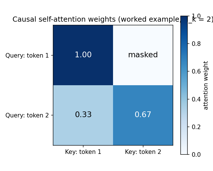
Causal attention weights from the worked example

বাংলা ব্যাখ্যা: ধাপগুলো মুখস্থ করো: স্কোর ($QK^\top$) → স্কেল ($\div\sqrt{d_k}$) → মাস্ক (ভবিষ্যৎ $-\infty$) → softmax → Value-র ওজন-গড়। প্রথম টোকেনের সামনে কেউ নেই, তাই তার ওজন (1, 0) — সে নিজের Value-ই কপি করে। দ্বিতীয় টোকেন দুজনকেই দেখে: ৩৩% নিজের আগেরটা, ৬৭% নিজে। $\sqrt{d_k}$ ভাগ না করলে স্কোর বড় হয়ে softmax জমে যায় (saturate), গ্রেডিয়েন্ট মরে যায় — এই তিন-ধাপ যুক্তিটাই "Explain why" উত্তর।

2.5.5 Multi-head attention¶

\[\operatorname{head}_i = \operatorname{Attention}(Q W_i^Q,\; K W_i^K,\; V W_i^V), \qquad \operatorname{MHA}(Q,K,V) = \operatorname{Concat}(\operatorname{head}_1, \dots, \operatorname{head}_h)\, W^O\]

With $h$ heads of size $d_k = d/h$ each, total compute matches one big head, but each head can specialize (syntax, coreference, positional patterns) — empirically better than a single head of the same total width.

2.5.6 The rest of the block¶

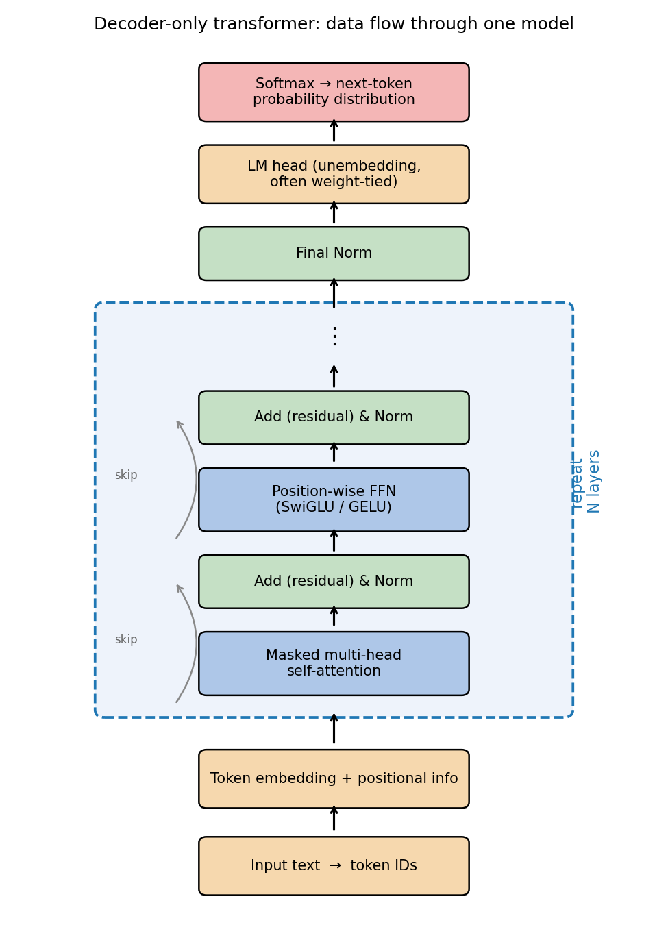
Residual connections: $y = x + \mathrm{Sublayer}(x)$ — gradients flow through the identity path; enables very deep stacks.
LayerNorm: $\mathrm{LN}(x) = \dfrac{x - \mu}{\sqrt{\sigma^2 + \varepsilon}} \cdot \gamma + \beta$ with mean $\mu$ and variance $\sigma^2$ computed per token across features; $\gamma, \beta$ learned. Tiny example: $x = (1, 3)$: $\mu = 2$, $\sigma^2 = 1$ → normalized $(-1.00, 1.00)$.
Feed-forward network (per position): $\mathrm{FFN}(x) = W_2 \,\phi(W_1 x)$, expansion factor ≈ 4 (e.g., 4096 → 16384 → 4096), activation GELU (classic) or SwiGLU (modern, Section 2.6). Holds most of the parameters; often interpreted as key-value memory for facts.
Output projection / LM head + weight tying: final hidden state × unembedding matrix → logits over the vocabulary. Tying the unembedding to the embedding matrix $E^\top$ saves $V \cdot d$ parameters and often improves perplexity.
Stacking: a model = embedding + $N$ identical blocks (e.g., 12, 32, 80) + final norm + LM head.

Decoder-only transformer data flow

2.5.7 Positional encoding (why and the sinusoidal how)¶

Self-attention is permutation-equivariant: shuffling the input tokens just shuffles the outputs — word order is invisible. Position must be injected explicitly.

Sinusoidal positional encoding (original transformer):

\[PE(pos, 2i) = \sin\!\left(\frac{pos}{10000^{2i/d}}\right), \qquad PE(pos, 2i+1) = \cos\!\left(\frac{pos}{10000^{2i/d}}\right)\]

Symbol	Meaning
$pos$	token position (0, 1, 2, …)
$i$	dimension-pair index; each pair $(2i, 2i{+}1)$ is one sinusoid frequency
$10000^{2i/d}$	wavelength — low dims oscillate fast, high dims slowly

Worked example ($d = 4$, $pos = 2$):

Pair $i = 0$: angle $= 2/10000^{0} = 2.00$ rad → $(\sin 2, \cos 2) = (0.91, -0.42)$.
Pair $i = 1$: angle $= 2/10000^{2/4} = 2/100 = 0.02$ rad → $(\sin 0.02, \cos 0.02) = (0.02, 1.00)$.

So $PE(2) = (0.91, -0.42, 0.02, 1.00)$, added to the token embedding. The multi-frequency design lets relative offsets be expressed as linear functions of the encodings; the lecture also notes the concern that adding position vectors to embeddings slightly distorts semantics — one motivation for RoPE (Section 2.6).

বাংলা ব্যাখ্যা: অ্যাটেনশন নিজে শব্দের ক্রম জানে না — "কুকুর মানুষকে কামড়াল" আর "মানুষ কুকুরকে কামড়াল" তার কাছে সমান! তাই প্রতিটি অবস্থানের জন্য আলাদা "অবস্থান-সংকেত" যোগ করা হয়। সাইন-কোসাইনের নানা ফ্রিকোয়েন্সি ব্যবহার করা হয় যাতে কাছের-দূরের সব স্কেলের দূরত্ব ধরা পড়ে — অনেকটা ঘড়ির সেকেন্ড-মিনিট-ঘণ্টার কাঁটার মতো।

2.5.8 NanoGPT and reading attention maps (lecture demo)¶

The lecture closes Section 2.5 with the NanoGPT example: a few hundred lines of code containing everything above — embedding table, causal self-attention, feed-forward network, residual + norm, stacked blocks, weight-tied LM head — proving that the conceptual parts list is complete.
Attention-map visualization: plotting the $(n, n)$ weight matrix of a trained head shows interpretable patterns — heads that attend to the previous token, heads that find matching brackets/quotes, heads that link pronouns to their referents.
How to read such a map in the exam: rows = query positions, columns = key positions, every row sums to 1.00, the upper triangle is empty in decoder-only models (causal mask). The heatmap of our worked example above is the 2×2 miniature of exactly this plot.

বাংলা ব্যাখ্যা: অ্যাটেনশন-ম্যাপ পড়ার নিয়ম: প্রতিটি সারি একটা টোকেনের "মনোযোগ-বাজেট" — যোগফল সবসময় ১। উপরের-ডান ত্রিভুজ ফাঁকা মানেই causal মাস্ক কাজ করছে। ট্রেনড মডেলে কিছু হেড আগের শব্দে, কিছু হেড মিলে-যাওয়া বন্ধনীতে, কিছু হেড সর্বনামের আসল মালিকে তাকায় — প্রতিটি হেড নিজের বিশেষ কাজ শিখে নেয়।

Code example — causal self-attention from scratch (numpy)¶

import numpy as np
def softmax(z, axis=-1):
    z = z - z.max(axis=axis, keepdims=True)
    e = np.exp(z); return e / e.sum(axis=axis, keepdims=True)

def causal_self_attention(Q, K, V):
    d_k = K.shape[-1]
    scores = Q @ K.T / np.sqrt(d_k)
    n = scores.shape[0]
    scores = np.where(np.triu(np.ones((n, n), bool), k=1), -1e9, scores)
    A = softmax(scores)
    return A @ V, A

Q = np.array([[1., 0.], [0., 1.]])
K = np.array([[1., 0.], [1., 1.]])
V = np.array([[1., 2.], [3., 4.]])
out, A = causal_self_attention(Q, K, V)
print(np.round(A, 2))    # [[1.   0.  ] [0.33 0.67]]
print(np.round(out, 2))  # [[1.   2.  ] [2.34 3.34]]

Common mistakes / exam traps¶

Forgetting the $\sqrt{d_k}$ scaling, or "scaling by $d_k$" (wrong — it is the square root).
Masking after the softmax (wrong — mask must be applied to scores before softmax so rows still sum to 1).
Confusing the attention matrix shape $(n, n)$ with the output shape $(n, d_v)$.
Saying attention has recurrence — it does not; that is exactly why it parallelizes.
Attention compute scales quadratically, $O(n^2 d)$, in context length $n$ — the cost driver for long contexts.

2.6 — Modern Transformer Variants¶

Same skeleton as 2.5, but every part has a "version 2" optimized for inference speed and quality: MHA → GQA → MQA (attention), GELU → SwiGLU (FFN), sinusoidal → RoPE (position), LayerNorm → RMSNorm (normalization).

2.6.1 The KV cache and why attention variants exist¶

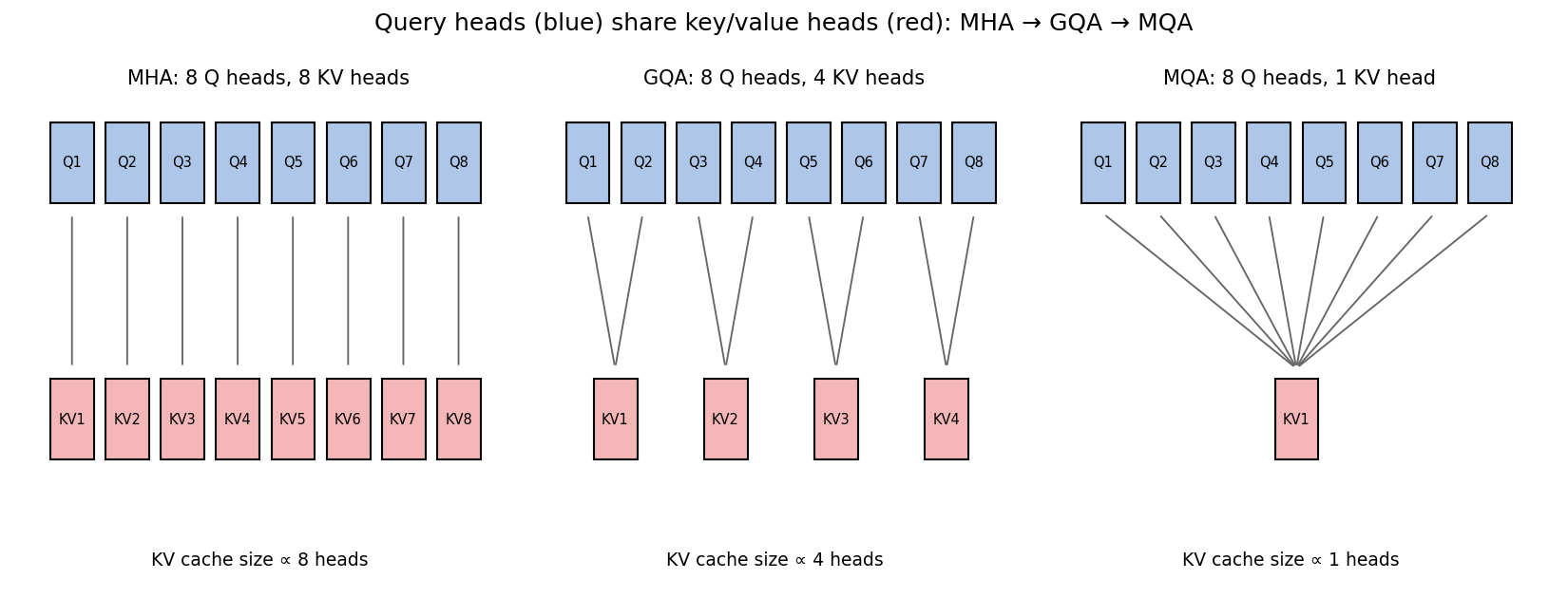
During generation, each new token needs the keys and values of all previous tokens. Recomputing them every step would cost $O(n^2)$ per token; instead they are stored in the KV cache. Its size (per layer, per token):

\[\text{KV bytes} = 2 \times n_{kv}\, \times d_{head} \times \text{bytes per value}\]

(the leading 2 = one K plus one V). Multi-/grouped-query attention shrink $n_{kv}$:

MHA: every one of the $h$ query heads has its own K/V head ($n_{kv} = h$).
GQA: query heads are partitioned into groups; each group shares one K/V head ($1 < n_{kv} < h$). Used by LLaMA-3.
MQA: all query heads share a single K/V head ($n_{kv} = 1$). Maximum saving, small quality loss.

Query heads sharing KV heads in MHA, GQA, MQA

Worked example — KV-cache size for a small config (2 decimals)¶

Config: 32 layers, 32 query heads, head dimension $d_{head} = 128$, FP16 storage (2 bytes), context length 8192.

Variant	$n_{kv}$	Bytes/token/layer $= 2 \cdot n_{kv} \cdot 128 \cdot 2$	Per token (×32 layers)	Full 8192 context
MHA	32	16,384 B = 16 KiB	512.00 KiB	4.00 GiB
GQA (8 groups)	8	4,096 B = 4 KiB	128.00 KiB	1.00 GiB
MQA	1	512 B = 0.5 KiB	16.00 KiB	0.12 GiB

GQA-8 gives a 4.00× reduction vs. MHA; MQA gives 32.00×. At a 128k context (131,072 tokens) the same model needs 64.00 GiB of KV cache with MHA — more than an entire 80 GB GPU after weights — but only 16.00 GiB with GQA-8 (see mock exam L4).

বাংলা ব্যাখ্যা: জেনারেশনের সময় প্রতিটি পুরোনো টোকেনের K আর V মেমোরিতে রাখতে হয় — এটাই KV ক্যাশ, আর লম্বা কনটেক্সটে এটাই মেমোরির সবচেয়ে বড় খরচ। GQA-র বুদ্ধি: প্রশ্ন-মাথা (Q) ৩২টাই থাক, কিন্তু উত্তর-মাথা (K/V) মাত্র ৮টা — কোয়ালিটি প্রায় same, মেমোরি ৪ ভাগের ১ ভাগ। MQA আরও চরম: সবার জন্য একটাই K/V।

2.6.2 SwiGLU activation in the FFN¶

\[\operatorname{FFN}_{\text{SwiGLU}}(x) \;=\; W_2\big(\operatorname{Swish}(W_1 x) \,\odot\, W_3 x\big), \qquad \operatorname{Swish}(z) = z \cdot \sigma(z)\]

Symbol	Meaning
$W_1, W_3$	two parallel up-projections (one gated, one gating)
$\odot$	element-wise product — the gate
$W_2$	down-projection back to model dimension

The multiplicative gate lets the network modulate information flow per dimension; empirically better loss than ReLU/GELU at equal parameter count (LLaMA, PaLM).

2.6.3 RoPE — Rotary Position Embedding¶

Instead of adding a position vector, RoPE rotates each 2-D pair of query/key components by an angle proportional to the absolute position:

\[\begin{pmatrix} x'_1 \\ x'_2 \end{pmatrix} = \begin{pmatrix} \cos m\theta_i & -\sin m\theta_i \\ \sin m\theta_i & \cos m\theta_i \end{pmatrix} \begin{pmatrix} x_1 \\ x_2 \end{pmatrix}, \qquad \theta_i = 10000^{-2i/d}\]

Symbol	Meaning
$m$	absolute position of the token
$\theta_i$	per-pair base frequency (like the sinusoidal wavelengths)
rotation	applied to $Q$ and $K$ only — not to $V$

Worked rotation: take the pair $(x_1, x_2) = (1, 0)$, position $m = 2$, frequency $\theta_0 = 1$:

\[x' = (\cos 2 \cdot 1 - \sin 2 \cdot 0,\;\; \sin 2 \cdot 1 + \cos 2 \cdot 0) = (-0.42,\; 0.91)\]

Why it is elegant — relative position for free: rotations preserve length, and the dot product of two rotated vectors depends only on the angle difference, i.e., on $m - n$:

\[\langle R_m q,\; R_n k \rangle = \langle q,\; R_{n-m} k \rangle\]

Numeric check (with $q = (1,1)$, $k = (0.5, -1)$, $\theta = 1$): rotate $q$ to position 3 and $k$ to position 1 → dot $= -1.16$; rotate $q$ to position 4 and $k$ to position 2 → dot $= -1.16$. Same offset (2), same score. ✔ Attention scores therefore encode relative distance — which generalizes better and supports context extension tricks.

বাংলা ব্যাখ্যা: RoPE অবস্থান-ভেক্টর যোগ করে না — Q আর K-কে ঘড়ির কাঁটার মতো ঘোরায়, যত দূরের টোকেন তত বেশি কোণ। ঘোরালে ভেক্টরের দৈর্ঘ্য বদলায় না, আর দুটো ঘোরানো ভেক্টরের ডট-প্রোডাক্ট নির্ভর করে শুধু কোণের পার্থক্যের ওপর — মানে শুধু "কত দূরে আছে" সেটার ওপর। উপরের সংখ্যা-পরীক্ষায় দেখো: অবস্থান (3,1) আর (4,2) — দুটোতেই স্কোর $-1.16$।

2.6.4 RMSNorm¶

\[\operatorname{RMSNorm}(x) = \frac{x}{\operatorname{RMS}(x)} \cdot \gamma, \qquad \operatorname{RMS}(x) = \sqrt{\tfrac{1}{d}\textstyle\sum_i x_i^2 + \varepsilon}\]

Drops LayerNorm's mean-subtraction and bias $\beta$ → fewer operations, empirically equal quality. Tiny example: $x = (3, 4)$: $\operatorname{RMS} = \sqrt{(9+16)/2} = \sqrt{12.5} = 3.54$ → output $(0.85, 1.13)\cdot\gamma$.

Code example — KV-cache parameter comparison¶

def kv_bytes_per_token(n_layers, n_kv_heads, d_head, bytes_per=2):
    return 2 * n_kv_heads * d_head * bytes_per * n_layers

for name, nkv in [("MHA", 32), ("GQA-8", 8), ("MQA", 1)]:
    per_tok = kv_bytes_per_token(32, nkv, 128)
    print(f"{name}: {per_tok/1024:.0f} KiB/token, "
          f"{per_tok*8192/2**30:.2f} GiB @ 8k ctx")
# MHA: 512 KiB/token, 4.00 GiB | GQA-8: 128 KiB, 1.00 GiB | MQA: 16 KiB, 0.12 GiB

Common mistakes¶

Saying GQA reduces parameter count significantly — its main win is KV-cache memory and bandwidth at inference.
Applying RoPE to V (it is applied to Q and K only).
Claiming RMSNorm normalizes across the batch — like LayerNorm it works per token across features.

2.7 — Decoding and Sampling Strategies¶

What the lecture says¶

Given the next-token distribution, how do we pick?

Greedy decoding: $w_t = \arg\max_w P(w \mid \text{prefix})$ — deterministic; often bland and repetitive (loops).
Pure sampling: $w_t \sim P$ — diverse but can pick from the low-quality long tail.
Temperature reshapes the distribution; top-k and top-p truncate it. Production chat systems typically combine temperature + top-p.

2.7.1 Softmax with temperature¶

\[P_i = \frac{\exp(z_i / T)}{\sum_j \exp(z_j / T)}\]

Symbol	Meaning
$z_i$	logit (raw score) of token $i$
$T$	temperature; $T \to 0$: argmax (greedy), $T < 1$: sharper, $T = 1$: unchanged, $T > 1$: flatter

Worked example — same 3 logits at three temperatures (2 decimals)¶

Logits $z = (2, 1, 0)$ for tokens A, B, C.

T = 1.0: $z/T = (2, 1, 0)$; $e^z = (7.39, 2.72, 1.00)$; sum $= 11.11$ → $P = (7.39/11.11,\; 2.72/11.11,\; 1.00/11.11) = (0.67, 0.24, 0.09)$.

T = 0.5 (sharper): $z/T = (4, 2, 0)$; $e^{z/T} = (54.60, 7.39, 1.00)$; sum $= 62.99$ → $P = (0.87, 0.12, 0.02)$. Top token gained mass: 0.67 → 0.87.

T = 2.0 (flatter): $z/T = (1, 0.5, 0)$; $e^{z/T} = (2.72, 1.65, 1.00)$; sum $= 5.37$ → $P = (0.51, 0.31, 0.19)$. Distribution approaches uniform.

As $T \to 0$, the gap $(z_1 - z_2)/T \to \infty$, so the softmax puts probability 1.00 on the argmax — greedy decoding as a limit (full argument in mock exam L2.3).

Same logits, three temperatures

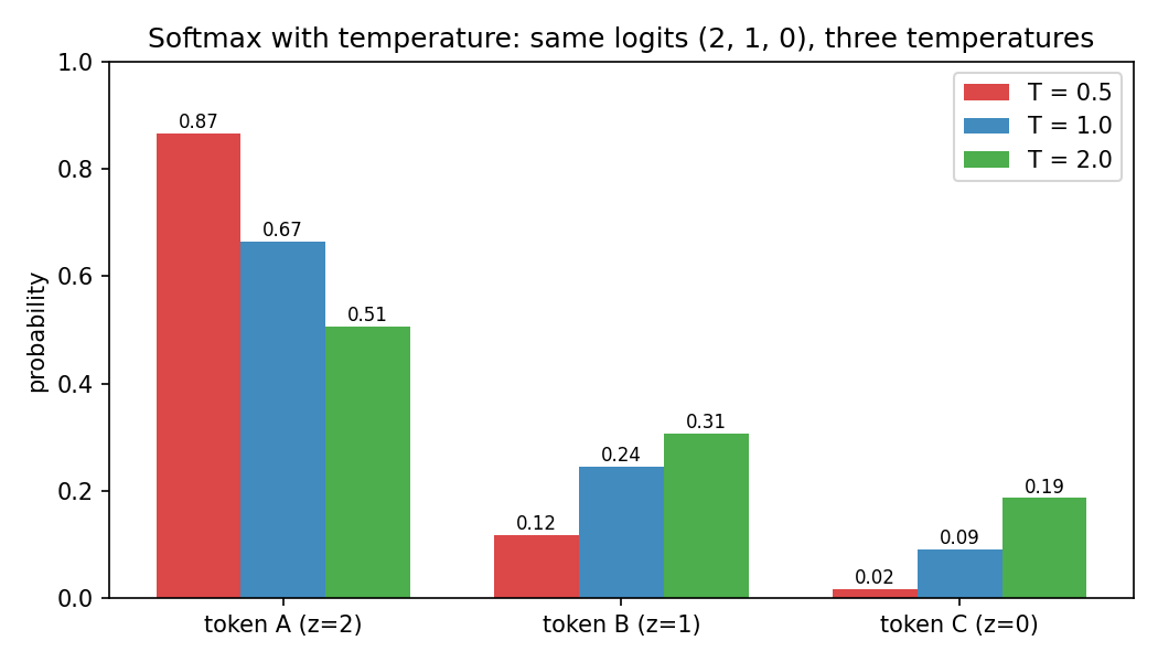
বাংলা ব্যাখ্যা: টেম্পারেচার হলো "ঝাল-নিয়ন্ত্রক"। T ছোট করলে logits-এর পার্থক্য বড় দেখায় → বিজয়ী টোকেন আরও নিশ্চিত (0.67 → 0.87) → আউটপুট একঘেয়ে কিন্তু নিরাপদ। T বড় করলে পার্থক্য চেপে যায় → সবাই কাছাকাছি সম্ভাবনা পায় (0.51/0.31/0.19) → সৃজনশীল কিন্তু ভুলের ঝুঁকি বেশি। T = 0 মানে সবসময় এক নম্বরটাই — সম্পূর্ণ deterministic।

2.7.2 Top-k and top-p (nucleus) — worked on one probability list¶

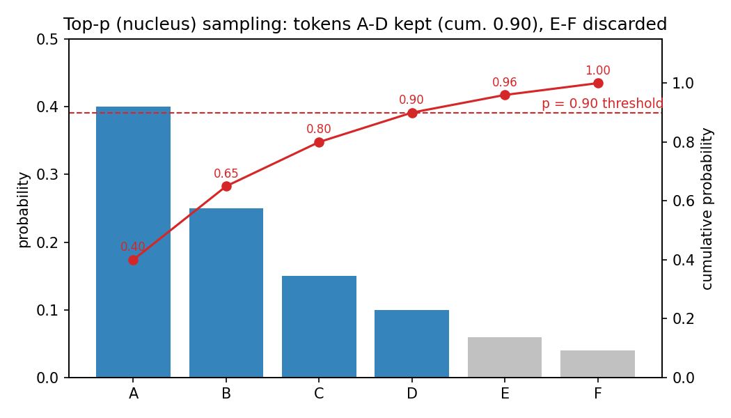
Sorted next-token distribution: A: 0.40, B: 0.25, C: 0.15, D: 0.10, E: 0.06, F: 0.04.

Top-k with k = 3: keep {A, B, C}, kept mass $= 0.40+0.25+0.15 = 0.80$. Renormalize by dividing by 0.80:

\[P' = (0.40/0.80,\; 0.25/0.80,\; 0.15/0.80) = (0.50,\; 0.31,\; 0.19)\]

Top-p with p = 0.90: cumulative sums: A: 0.40 → B: 0.65 → C: 0.80 → D: 0.90 ✔ (threshold reached). Keep the smallest prefix whose cumulative mass ≥ 0.90: {A, B, C, D}, mass 0.90. Renormalize by 0.90:

\[P' = (0.44,\; 0.28,\; 0.17,\; 0.11)\]

E and F (the unreliable tail) are eliminated in both cases.

Key difference (classic MC question): top-k keeps a fixed count regardless of distribution shape; top-p keeps an adaptive set — when the model is confident (peaked distribution) the nucleus may contain only 1–2 tokens, and when it is uncertain (flat distribution) the nucleus widens. Edge case: if the top token alone has probability ≥ p, top-p keeps just that single token (handled in mock exam L5.2).

Top-p cumulative cutoff at p = 0.90

বাংলা ব্যাখ্যা: top-k বলে "সেরা k-জনকে রাখো" — বিতরণ যেমনই হোক, সংখ্যাটা fixed। top-p বলে "জমা সম্ভাবনা p% না ছোঁয়া পর্যন্ত রাখতে থাকো" — মডেল নিশ্চিত থাকলে হয়তো ১টা টোকেনই থাকে, দ্বিধায় থাকলে অনেকগুলো। দুটোরই লক্ষ্য এক: লেজের আবর্জনা-টোকেন বাদ দেওয়া। বাদ দেওয়ার পর বাকিগুলোকে আবার যোগফল-১ করতে ভাগ (renormalize) করতে হয় — পরীক্ষায় এই ধাপ ভুললে নম্বর কাটা।

Code example — all four strategies¶

import numpy as np
def temperature(logits, T):
    z = logits / T; z -= z.max(); e = np.exp(z); return e / e.sum()
def top_k(p, k):
    idx = np.argsort(p)[-k:]; q = np.zeros_like(p); q[idx] = p[idx]; return q / q.sum()
def top_p(p, pp):
    order = np.argsort(p)[::-1]
    cum = np.cumsum(p[order])
    cutoff = int(np.searchsorted(cum, pp)) + 1     # smallest set with cum >= pp
    keep = order[:cutoff]
    q = np.zeros_like(p); q[keep] = p[keep]; return q / q.sum()

probs = np.array([0.40, 0.25, 0.15, 0.10, 0.06, 0.04])
print(np.round(top_k(probs, 3), 2))    # [0.5  0.31 0.19 0.   0.   0.  ]
print(np.round(top_p(probs, 0.9), 2))  # [0.44 0.28 0.17 0.11 0.   0.  ]

When to use what (application-question ammunition)¶

Setting	Recommendation	Justification	Trade-off
Factual QA, extraction, code	greedy or T ≈ 0–0.3	reproducible, fewest hallucinated tokens	repetitive, no diversity
Chat assistant	T ≈ 0.7 + top-p 0.90	natural variety, tail cut off	mild nondeterminism
Creative writing, brainstorming	T ≈ 1.0–1.3 + top-p	exploration of unlikely continuations	more incoherence risk

2.8 — Pretraining¶

What the lecture says¶

Objective: next-token prediction with cross-entropy loss over a web-scale corpus (self-supervised — the text itself provides the labels).
Hardware: GPUs do massive parallel matrix multiplications (10–100× CPU throughput); frontier training runs use thousands of H100/H200-class accelerators. LLaMA-3.1-405B: ~15 T tokens, ~30 M GPU-hours.
Precision formats: FP32 → FP16/BF16 (mixed precision) → FP8. Lower precision halves memory traffic and roughly doubles throughput; BF16 keeps FP32's exponent range (no loss scaling drama).
Batching and gradient accumulation, learning-rate schedules (warmup + cosine decay), AdamW optimizer, distributed training (data / tensor / pipeline parallelism, ZeRO/FSDP sharding).

2.8.1 Cross-entropy training objective¶

\[\mathcal{L}(\theta) = -\frac{1}{T}\sum_{t=1}^{T} \log P_\theta\!\left(w_t \mid w_{<t}\right)\]

Symbol	Meaning
$\theta$	model parameters
$T$	number of token positions in the batch
$w_t$	the true next token at position $t$
$P_\theta(w_t \mid w_{<t})$	probability the model assigned to the true token

Perplexity $= e^{\mathcal{L}}$ (Section 2.12 works this out numerically).

2.8.2 Compute cost — the 6ND rule, worked¶

\[C \;\approx\; 6\, N\, D \quad \text{FLOPs}\]

Symbol	Meaning
$N$	number of parameters
$D$	number of training tokens
6	≈ 2 FLOPs/param for the forward pass + ≈ 4 for the backward pass, per token

Worked example: train a $N = 7\times10^9$ parameter model on $D = 140\times10^9$ tokens (the Chinchilla-optimal 20:1 ratio):

\[C = 6 \times (7\times10^9) \times (1.4\times10^{11}) = 5.88\times10^{21} \ \text{FLOPs}\]

At a sustained $10^{15}$ FLOP/s per GPU (H100-class with good utilization):

\[\frac{5.88\times10^{21}}{10^{15}} = 5.88\times10^{6}\ \text{s} = 68.06 \ \text{GPU-days} \;\;\Rightarrow\;\; \approx 8.51\ \text{days on 8 GPUs}.\]

বাংলা ব্যাখ্যা: 6ND হলো ট্রেনিং খরচের পকেট-ক্যালকুলেটর: প্রতি টোকেনে প্রতি প্যারামিটারে forward-এ ~২টা আর backward-এ ~৪টা গুণ-যোগ — মোট ৬। N আর D গুণ করে ৬ দিয়ে গুণ দিলেই মোট FLOPs। তারপর GPU-র গতি দিয়ে ভাগ দিলে সময়। পরীক্ষায় এই হিসাব scientific notation-এ পরিষ্কারভাবে দেখাতে হবে।

2.8.3 Gradient accumulation — effective batch size, worked¶

GPU memory limits the micro-batch per device. Gradients are summed over $k$ micro-batches before one optimizer step:

\[B_{\text{eff}} = b_{\text{micro}} \times k_{\text{accum}} \times n_{\text{GPUs}}\]

Worked example: $b_{\text{micro}} = 4$ sequences, $k_{\text{accum}} = 16$, $n_{\text{GPUs}} = 8$:

\[B_{\text{eff}} = 4 \times 16 \times 8 = 512 \ \text{sequences per optimizer step}\]

Mathematically identical to one big batch of 512 (gradients are linear/averageable); the price is wall-clock time, not correctness.

2.8.4 Optimizer memory — worked GB numbers¶

Adam(W) keeps two extra statistics per parameter (first moment $m$, second moment $v$). For an $N = 7\times10^9$ model with standard mixed-precision training:

Component	Bytes/param	Total for 7 B
FP16 working weights	2	14.00 GB
FP16 gradients	2	14.00 GB
FP32 master weights	4	28.00 GB
FP32 Adam first moment $m$	4	28.00 GB
FP32 Adam second moment $v$	4	28.00 GB
Total training state	16	112.00 GB

So training a 7 B model needs ≈ 112.00 GB of state (before activations!) — does not fit on one 80 GB GPU → ZeRO/FSDP shard these states across devices. Inference in FP16 needs only $2 \times 7\times10^9 = $ 14.00 GB. The 16-bytes-per-parameter rule of thumb is exam gold.

বাংলা ব্যাখ্যা: ট্রেনিং-এ শুধু ওজন রাখলেই হয় না — গ্রেডিয়েন্ট, FP32 মাস্টার-কপি, আর Adam-এর দুই মোমেন্ট ($m$, $v$) মিলে প্যারামিটার-প্রতি ~১৬ বাইট লাগে। তাই ৭B মডেল চালাতে ১৪ GB লাগলেও ট্রেন করতে লাগে ১১২ GB — এই ৮ গুণ ফারাকটাই বুঝিয়ে দেয় কেন fine-tuning-এর জন্য LoRA-র মতো কৌশল দরকার (অধ্যায় ৬-এর পূর্বাভাস)।

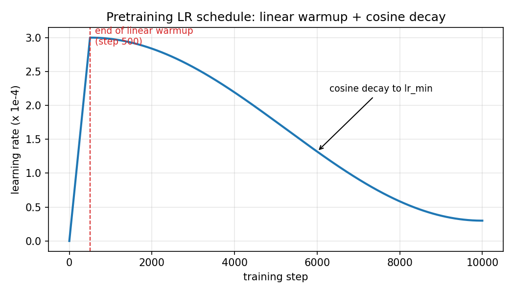
2.8.5 Learning-rate schedule: warmup + cosine decay¶

Linear warmup (e.g., first 500–2000 steps): Adam's moment estimates and the loss surface are unreliable at step 0; a large early LR can destabilize/diverge the run. Ramping up avoids this.
Cosine decay to ~10% of peak: large steps early for fast progress, small steps late for fine convergence.

Linear warmup followed by cosine decay

Code example — tiny training loop with gradient accumulation¶

import torch, torch.nn as nn, torch.nn.functional as F
model = nn.Sequential(nn.Embedding(50, 32), nn.Linear(32, 50))
opt = torch.optim.AdamW(model.parameters(), lr=3e-3)
data = torch.randint(0, 50, (1024, 17))
ACCUM = 4
for step in range(100):
    opt.zero_grad()
    for micro in range(ACCUM):                       # gradient accumulation
        idx = torch.randint(0, 1024, (8,))
        x, y = data[idx, :-1], data[idx, 1:]
        logits = model[1](model[0](x))
        loss = F.cross_entropy(logits.reshape(-1, 50), y.reshape(-1)) / ACCUM
        loss.backward()                              # gradients sum up
    opt.step()                                       # one step per 4 micro-batches

Common mistakes¶

Using 2ND (forward only) instead of 6ND for training cost.
Saying gradient accumulation saves compute — it saves memory; FLOPs are unchanged.
Forgetting that Adam state ≈ 2 extra FP32 copies — the reason "training needs ~8× inference memory".

2.9 — In-Context Learning¶

What the lecture says¶

A pretrained LLM can perform new tasks at inference time purely from the prompt — no parameter update.
Zero-shot: instruction only. Few-shot: instruction + a handful of input→output examples.
Mechanism (lecture's framing): the examples let the model recognize a task pattern it has implicitly learned during pretraining and continue that pattern for the new input. In-context "learning" is pattern completion, not gradient descent.
Emergent with scale: small models barely benefit from examples; large models do strikingly.

prompt = """Translate to French:
English: cat   -> French: chat
English: dog   -> French: chien
English: book  -> French:"""        # model continues: " livre"

বাংলা ব্যাখ্যা: এখানে মডেলের ওজন এক বিটও বদলায় না — প্রম্পটের উদাহরণগুলো দেখে মডেল বুঝে নেয় "ও আচ্ছা, এটা অনুবাদের খেলা", তারপর প্যাটার্নটা চালিয়ে যায়। এটা গ্রেডিয়েন্ট-শেখা নয়, প্যাটার্ন-চেনা। অধ্যায় ৩-এর সব প্রম্পটিং-কৌশল (few-shot, chain-of-thought) এই ক্ষমতারই প্রয়োগ।

In-context learning vs. fine-tuning (application-question table)¶

Axis	In-context learning	Fine-tuning (Chapter 6)
What changes	nothing — only the prompt	the model weights
Cost per task	zero setup; pay per prompt token at every call	one-time training cost; cheap at call time
Number of examples	limited by the context window	unlimited (whole datasets)
Persistence	gone when the prompt ends	permanent skill
Best when	few examples, fast iteration, many ad-hoc tasks	stable task, large data, strict latency/cost budget
Risk	examples eat context budget; sensitive to example choice/order	overfitting, catastrophic forgetting, infra effort

Exam relevance¶

Contrast in-context learning vs. fine-tuning: prompt-time vs. weight-update; no training cost vs. permanent skill; context-window-limited vs. unlimited examples.
Application-question trade-off: few-shot examples consume context tokens (cost + latency) but need no training infrastructure.
Zero-shot vs. few-shot: instruction only vs. instruction plus input→output demonstrations; few-shot gains are an emergent property of scale.

2.10 — Alignment: SFT, RLHF, DPO¶

What the lecture says¶

A pretrained model is a completion engine — fluent but not helpful, harmless, or honest ("What is the capital of France?" may be continued with more exam questions rather than an answer). Post-training fixes this in stages: Pretraining → Supervised Fine-Tuning → Preference Optimization (RLHF or DPO).

বাংলা ব্যাখ্যা: প্রিট্রেইনড মডেল শুধু "পরের শব্দ" জানে — প্রশ্ন করলে উত্তর না দিয়ে আরও প্রশ্ন বানাতে পারে! তাই দুই ধাপ শোধন: প্রথমে SFT — আদর্শ উত্তর দেখিয়ে "সহকারীর ভূমিকা" শেখানো; তারপর preference tuning — দুটো উত্তরের মধ্যে কোনটা মানুষ বেশি পছন্দ করে, সেই সংকেতে আরও ঘষামাজা।

2.10.1 Supervised Fine-Tuning (SFT)¶

Train on curated (instruction $x$, ideal answer $y$) pairs with the same cross-entropy loss as pretraining, but only over answer tokens:

\[\mathcal{L}_{\text{SFT}}(\theta) = -\,\mathbb{E}_{(x, y)\sim \mathcal{D}_{\text{SFT}}} \sum_{t} \log \pi_\theta\!\left(y_t \mid x,\, y_{<t}\right)\]

Symbol	Meaning
$\pi_\theta$	the model viewed as a policy (token distribution given context)
$\mathcal{D}_{\text{SFT}}$	dataset of demonstration pairs
$y_t,\ y_{<t}$	answer token at step $t$ and its prefix

Limitation (exam-critical): SFT only shows good answers — it carries no signal about better vs. worse, cannot express "this answer is acceptable but that one is preferable", and the model only imitates the demonstrators' ceiling.

2.10.2 RLHF — reward model + KL-regularized RL¶

Step 1 — collect preferences: humans see a prompt and two candidate answers, pick the better one → triples $(x, y_w, y_l)$ (winner/loser).

Step 2 — train a reward model $r_\phi(x, y)$ with the Bradley–Terry model of pairwise preference:

\[P(y_w \succ y_l \mid x) = \sigma\big(r_\phi(x, y_w) - r_\phi(x, y_l)\big), \qquad \mathcal{L}_{\text{RM}}(\phi) = -\,\mathbb{E}\big[\log \sigma\big(r_\phi(x, y_w) - r_\phi(x, y_l)\big)\big]\]

Symbol	Meaning
$r_\phi$	scalar reward head on an LLM backbone; parameters $\phi$
$\sigma(z) = 1/(1+e^{-z})$	sigmoid: maps reward gap to win probability
$y_w, y_l$	human-preferred and rejected answer

Step 3 — optimize the policy with PPO against the reward, leashed to a frozen reference:

\[\max_\theta \;\; \mathbb{E}_{x \sim \mathcal{D},\, y \sim \pi_\theta} \Big[ r_\phi(x, y) \Big] \;-\; \beta \, \mathbb{D}_{\mathrm{KL}}\!\big(\pi_\theta(\cdot \mid x)\,\big\|\,\pi_{\text{ref}}(\cdot \mid x)\big)\]

Symbol	Meaning
$\pi_\theta$	the policy being trained (the LLM)
$\pi_{\text{ref}}$	frozen post-SFT reference model
$\beta$	KL-penalty strength: how far the policy may drift from the reference
$\mathbb{D}_{\mathrm{KL}}$	Kullback–Leibler divergence — penalizes distribution drift

Why the KL term is essential: the reward model is an imperfect proxy. Without the leash, the policy finds adversarial outputs that score high reward but are degenerate (reward hacking: sycophantic, repetitive, verbose text) and loses linguistic diversity (mode collapse). The KL term anchors the policy to fluent SFT behavior.

PPO clipped objective (the inner RL machinery):

\[\mathcal{L}^{\text{CLIP}}(\theta) = \mathbb{E}\Big[\min\big(\rho_t A_t,\;\; \operatorname{clip}(\rho_t,\, 1-\epsilon,\, 1+\epsilon)\, A_t\big)\Big], \qquad \rho_t = \frac{\pi_\theta(a_t \mid s_t)}{\pi_{\theta_{\text{old}}}(a_t \mid s_t)}\]

with advantage $A_t$ and clip width $\epsilon$ (≈ 0.2) — the clip prevents destructively large policy updates.

বাংলা ব্যাখ্যা: RLHF তিন ধাপ: (১) মানুষ দুটো উত্তরের মধ্যে ভালোটা বাছে; (২) সেই পছন্দ থেকে একটা reward model শেখে — Bradley–Terry সূত্রে reward-এর পার্থক্য জেতার সম্ভাবনা ঠিক করে; (৩) PPO দিয়ে মূল মডেলকে reward বাড়াতে শেখানো হয়, কিন্তু KL-দড়ি দিয়ে রেফারেন্স মডেলের সাথে বেঁধে রাখা হয়। দড়ি না থাকলে মডেল reward model-কে "ঠকানোর" পথ খুঁজে নেয় — তোষামুদে, ফাঁপা লম্বা উত্তর — এটাই reward hacking।

2.10.3 DPO — Direct Preference Optimization¶

Key insight: the KL-regularized RL problem above has a closed-form optimal policy, and substituting it back turns the preference objective into a simple supervised loss on the policy itself — no reward model, no RL loop:

\[\mathcal{L}_{\text{DPO}}(\theta) = -\,\mathbb{E}_{(x, y_w, y_l)}\left[\log \sigma\!\left(\beta \log \frac{\pi_\theta(y_w \mid x)}{\pi_{\text{ref}}(y_w \mid x)} \;-\; \beta \log \frac{\pi_\theta(y_l \mid x)}{\pi_{\text{ref}}(y_l \mid x)}\right)\right]\]

What each term does:

Term	Role
$\log \frac{\pi_\theta(y_w \mid x)}{\pi_{\text{ref}}(y_w \mid x)}$	implicit reward of the winner: how much more likely the policy makes $y_w$ relative to the reference
$\log \frac{\pi_\theta(y_l \mid x)}{\pi_{\text{ref}}(y_l \mid x)}$	implicit reward of the loser — pushed down relative to reference
difference of the two	implicit reward margin; the loss wants it large and positive
$\beta$	temperature of the implicit reward ≈ inverse KL strength: small $\beta$ = stay close to reference
$\log \sigma(\cdot)$	Bradley–Terry log-likelihood — exactly the reward-model loss, but with the policy's own log-ratios playing the reward role

Gradient intuition: $\nabla\mathcal{L} \propto -(1 - \sigma(\text{margin})) \cdot [\nabla \log \pi_\theta(y_w) - \nabla \log \pi_\theta(y_l)]$ — increase the winner's log-probability, decrease the loser's, with force proportional to how wrong the current margin is.

import torch, torch.nn.functional as F
def dpo_loss(logp_w, logp_l, ref_w, ref_l, beta=0.1):
    margin = beta * ((logp_w - ref_w) - (logp_l - ref_l))
    return -F.logsigmoid(margin).mean()
# toy numbers: logp_w=-1.0, logp_l=-1.5, ref_w=-1.2, ref_l=-1.4
# margin = 0.1*((-1.0+1.2) - (-1.5+1.4)) = 0.1*(0.2+0.1) = 0.03 -> loss = 0.68

বাংলা ব্যাখ্যা: DPO-র চালাকি: আলাদা reward model বানানোর দরকারই নেই — পলিসির নিজের লগ-সম্ভাবনা আর রেফারেন্সের অনুপাতটাই "লুকানো reward" হিসেবে কাজ করে। লস চায় বিজয়ী উত্তরের অনুপাত বাড়ুক, পরাজিতেরটা কমুক। ফলে RLHF-এর ৪টা মডেল (policy, reference, reward, critic) জাগলিং করার বদলে একটা সাধারণ supervised লসেই কাজ হয়ে যায় — সস্তা ও স্থিতিশীল।

2.10.4 SFT vs. RLHF vs. DPO — qualitative comparison¶

Axis	SFT	RLHF (PPO)	DPO
Training signal	ideal demonstrations only	pairwise preferences via learned reward	pairwise preferences directly
Expresses "better vs. worse"?	no	yes	yes
Extra models needed	none	reward model + value/critic + reference	reference only
Optimization	supervised cross-entropy (stable)	reinforcement learning loop (unstable, many hyperparameters)	supervised logistic-style loss (stable)
Compute / engineering cost	low	very high (sampling + 4 models in memory)	moderate
Exploration beyond data	none (imitation ceiling)	yes — can discover responses better than any demonstration	limited — bound to offline preference pairs
Main failure modes	imitates demonstrator errors	reward hacking, mode collapse, over-refusal, sycophancy	overfits preference set; implicit reward mis-generalizes off-distribution
Typical role today	step 1 (always)	step 2 at frontier labs	step 2 for most open-source models

Other lecture points: human preference disagreement (annotators disagree; "aligned to whom?" is unsolved); alignment failure modes: sycophancy (agreeing with the user over truth), mode collapse (loss of output diversity), over-refusal, reward hacking.

Common mistakes¶

"DPO has no KL control" — wrong: $\beta$ is the KL knob, and $\pi_{\text{ref}}$ appears explicitly in the loss.
"RLHF trains on demonstrations" — no, on preferences; demonstrations belong to SFT.
Forgetting why $\pi_{\text{ref}}$ exists at all (anchor against reward hacking / distribution drift).

2.11 — Scaling Laws¶

What the lecture says¶

Empirically, validation loss falls predictably with scale:

\[L(N, D) \;=\; E \;+\; \frac{A}{N^{\alpha}} \;+\; \frac{B}{D^{\beta}}\]

Symbol	Meaning
$N$	parameters; $D$ — training tokens
$E$	irreducible loss (entropy of language itself)
$A/N^\alpha$	error from limited model capacity
$B/D^\beta$	error from limited data

Loss improvements are smooth power laws — predictable, but each halving of loss needs ~10× more compute.
Chinchilla result: for a fixed compute budget $C \approx 6ND$, the loss-optimal allocation scales $N$ and $D$ together, with approximately $$D^* \;\approx\; 20\, N^*$$ (20 training tokens per parameter). GPT-3 (175 B params, 300 B tokens ≈ 1.7 tokens/param) was badly under-trained for its size.

Worked example — given compute $C$, find $N^$ and $D^$¶

Problem: budget $C = 1\times10^{21}$ FLOPs. Using $C = 6ND$ and the Chinchilla condition $D = 20N$, find the optimal $N$ and $D$.

Step 1 — substitute: $C = 6N(20N) = 120\,N^2$.

Step 2 — solve for N:

\[N^* = \sqrt{\frac{C}{120}} = \sqrt{\frac{10^{21}}{120}} = \sqrt{8.33\times10^{18}} = 2.89\times10^{9} \approx 2.89\ \text{B parameters}\]

Step 3 — tokens: $D^* = 20 N^* = 5.77\times10^{10} \approx 57.74\ \text{B tokens}$.

Check: $6 \times 2.89\times10^9 \times 5.77\times10^{10} = 1.00\times10^{21}$. ✔

Compute-optimal ≠ deployment-optimal (exam favorite): Chinchilla optimizes training loss per training FLOP. But inference cost scales with $N$, and a model is run many more times than it is trained. Hence labs deliberately over-train small models far beyond 20 tokens/param (LLaMA-3-8B: ~15 T tokens ≈ 1875 tokens/param) — slightly worse than the compute-optimal training trade, much cheaper to serve.

বাংলা ব্যাখ্যা: Chinchilla-র বার্তা: কম্পিউট বাজেট থাকলে মডেল আর ডেটা একসাথে বাড়াও — প্রতি প্যারামিটারে ~২০ টোকেন। হিসাবের কৌশল: $D = 20N$ বসিয়ে দিলে $C = 120N^2$, তারপর বর্গমূল। কিন্তু খেয়াল রেখো — এটা শুধু ট্রেনিং-খরচের অপটিমাম; বাস্তবে মডেল কোটি কোটি বার চালানো হয়, তাই ছোট মডেলকে ইচ্ছা করে ২০-র বহু গুণ বেশি টোকেনে ট্রেন করা হয় যাতে সার্ভ করা সস্তা হয়। "LLaMA কেন Chinchilla-optimal নয়?" — এই প্রশ্নের উত্তর এটাই।

import math
C = 1e21
N = math.sqrt(C / 120)        # 2.89e9 parameters
D = 20 * N                    # 5.77e10 tokens
print(f"N*={N:.2e}, D*={D:.2e}, check 6ND={6*N*D:.2e}")

Common mistakes¶

Treating 20 tokens/param as a law of nature — it is an empirical fit under specific assumptions.
Confusing compute-optimal (training) with cost-optimal (lifetime = training + inference).
Saying scaling laws guarantee specific capabilities — they predict loss, not skills.

2.12 — Evaluation¶

What the lecture says¶

Intrinsic evaluation: cross-entropy / perplexity on held-out text. Cheap, smooth, ideal for tracking pretraining — but not user-facing and tokenizer-dependent (not comparable across different vocabularies).
Task metrics: BLEU/ROUGE (translation/summarization n-gram overlap), exact match / F1 (QA), pass@k (code: probability ≥ 1 of k samples passes unit tests).
Capability benchmarks: MMLU (broad knowledge MC), GSM-8K (grade-school math), HumanEval (code), MultiChallenge (multi-turn instruction following), Tau-2 (tool use/agents).
Safety evaluation: red-teaming, ToxicChat, jailbreak resistance.
Benchmark limitations: contamination (test data in training data — a data-side problem), saturation, overfitting-to-the-leaderboard (gaming), weak correlation with real user value → also use human preference arenas and task-specific evals.

Perplexity — definition and worked example (nats and bits)¶

\[H = -\frac{1}{T}\sum_{t=1}^{T} \log P_\theta(w_t \mid w_{<t}), \qquad \mathrm{PPL} = e^{H} \;\;(\text{natural log}) \;=\; 2^{H_2}\;\;(\text{log base 2})\]

Worked example: the model assigned the true next tokens probabilities $0.50,\ 0.25,\ 0.125,\ 0.50$.

In nats (natural log):

token prob	$-\ln p$
0.50	0.69
0.25	1.39
0.125	2.08
0.50	0.69

\[H = \frac{0.69 + 1.39 + 2.08 + 0.69}{4} = \frac{4.85}{4} = 1.21 \ \text{nats} \qquad \mathrm{PPL} = e^{1.21} = 3.36\]

In bits (log base 2): $-\log_2 p = 1, 2, 3, 1$ → $H_2 = 7/4 = 1.75$ bits → $\mathrm{PPL} = 2^{1.75} = 3.36$. Same perplexity, as it must be — perplexity is base-independent.

Interpretation: the model is, on average, as uncertain as a fair choice among 3.36 equally likely tokens ("effective branching factor"). Lower is better; PPL = 1 would be perfect prediction.

বাংলা ব্যাখ্যা: Perplexity মানে "মডেল গড়ে কয়টা অপশনের মধ্যে দ্বিধায় আছে"। হিসাবের রেসিপি: সত্যিকারের টোকেনগুলোর সম্ভাবনার $-\log$ নাও, গড় করো (এটাই cross-entropy), তারপর exponential — $e$ দিয়ে করলে ন্যাটস, ২ দিয়ে করলে বিটস, কিন্তু শেষ PPL একই। PPL 3.36 মানে মডেল যেন প্রতিবার ৩.৩৬টা সমান-সম্ভাব্য টোকেনের মধ্যে আন্দাজ করছে।

Benchmark overview (memorize what each one measures)¶

Benchmark	Measures	Format
MMLU	broad academic/world knowledge, 57 subjects	multiple choice
GSM-8K	grade-school multi-step math reasoning	free-form numeric answer
HumanEval	code generation correctness	unit tests, scored with pass@k
MultiChallenge	multi-turn instruction following	conversational tasks
Tau-2	tool use / agentic behavior	simulated tool-calling environments
ToxicChat / red-teaming	safety, jailbreak resistance	adversarial prompts

বাংলা ব্যাখ্যা: প্রতিটি বেঞ্চমার্ক একেকটা আলাদা পেশি মাপে — MMLU জ্ঞান, GSM-8K গণিত-যুক্তি, HumanEval কোড, Tau-2 টুল-ব্যবহার। কিন্তু মনে রেখো চার দুর্বলতা: contamination (প্রশ্ন আগেই দেখা), saturation (সবাই ~১০০% পেয়ে গেলে আর পার্থক্য ধরা যায় না), gaming (লিডারবোর্ডের জন্য টিউন করা), আর বাস্তব-উপযোগিতার সাথে দুর্বল সম্পর্ক।

Code example — pass@k¶

import math
def pass_at_k(n, c, k):
    """P(>=1 correct in k draws) given c correct among n samples."""
    if n - c < k:
        return 1.0
    return 1 - math.comb(n - c, k) / math.comb(n, k)
print(round(pass_at_k(100, 20, 1), 2))    # 0.20
print(round(pass_at_k(100, 20, 10), 2))   # 0.91

Common mistakes¶

Comparing perplexities of models with different tokenizers (not meaningful).
Calling contamination a model defect — it is a training-data defect; the fix is decontamination of the corpus.
Assuming a higher MMLU score always means a better assistant (benchmarks ≠ user value).

Chapter Cheat Sheet¶

Formulas (memorize, with symbols):

Name	Formula
Cross-entropy loss	$\mathcal{L} = -\frac{1}{T}\sum_t \log P_\theta(w_t \mid w_{<t})$
Perplexity	$\mathrm{PPL} = e^{\mathcal{L}}$ (nats) $= 2^{H_2}$ (bits)
Softmax + temperature	$P_i = e^{z_i/T} / \sum_j e^{z_j/T}$
Attention	$\operatorname{softmax}(QK^\top / \sqrt{d_k})\,V$
Multi-head	$\operatorname{Concat}(\text{heads})\,W^O$, $d_k = d/h$
Cosine similarity	$u\cdot v / (\lVert u\rVert \lVert v\rVert)$; unit vectors: $\lVert\hat u - \hat v\rVert^2 = 2 - 2\cos$
Sinusoidal PE	$\sin / \cos(pos / 10000^{2i/d})$
KV cache	$2 \cdot n_{kv} \cdot d_{head} \cdot \text{bytes} \cdot n_{layers} \cdot n_{ctx}$
Training FLOPs	$C \approx 6ND$
Chinchilla	$D^* \approx 20N^$ → with $C = 6ND$: $N^ = \sqrt{C/120}$
Adam training memory	≈ 16 bytes/param (weights, grads, master, $m$, $v$)
Bradley–Terry	$P(y_w \succ y_l) = \sigma(r_w - r_l)$
RLHF objective	$\max\ \mathbb{E}[r_\phi] - \beta\,\mathbb{D}_{\mathrm{KL}}(\pi_\theta \\| \pi_{\text{ref}})$
DPO loss	$-\log\sigma(\beta[\log\frac{\pi_\theta(y_w)}{\pi_{\text{ref}}(y_w)} - \log\frac{\pi_\theta(y_l)}{\pi_{\text{ref}}(y_l)}])$

Quick numbers: 1 token ≈ 0.75 English words · LLaMA-3: 128k vocab, 15 T tokens, GQA-8 · attention cost $O(n^2 d)$ · warmup → cosine decay · PPO clip ε ≈ 0.2 · pass@k for code.

Top traps: 1. Forgetting $\sqrt{d_k}$ (and it is the square root, not $d_k$). 2. Masking after softmax instead of before. 3. Cosine vs. Euclidean disagree on unnormalized vectors; agree in ranking after L2 normalization. 4. Top-k = fixed count; top-p = adaptive mass; both need renormalization. 5. Gradient accumulation saves memory, not FLOPs. 6. Chinchilla-optimal ≠ deployment-optimal (LLaMA over-trains on purpose). 7. SFT learns from demonstrations; RLHF/DPO learn from preferences. 8. Perplexity is tokenizer-dependent; contamination is a data-side problem.

Difficult English ↔ বাংলা: alignment → মূল্যবোধ-সমন্বয়; supervised → তত্ত্বাবধানে; preference → পছন্দ; reward → পুরস্কার; logit → softmax-এর আগের কাঁচা স্কোর; hallucination → বানোয়াট তথ্য; deduplication → পুনরাবৃত্তি-অপসারণ; saturation → জমে যাওয়া/সম্পৃক্তি।

Rapid-fire self-check (cover the right column):

Prompt	One-line answer
Why sub-word instead of word tokenization?	bounded vocabulary + no out-of-vocabulary, short sequences for frequent strings
What does the embedding matrix's row $i$ contain?	the learned vector of token $i$ (one-hot times $E$)
Cosine of orthogonal vectors?	0.00
Unit vectors: relation distance ↔ cosine?	$\lVert\hat u-\hat v\rVert^2 = 2 - 2\cos$ → same ranking
Order of attention steps?	scores → scale → mask → softmax → weighted sum of values
Shape of attention weights / output?	$(n, n)$ / $(n, d_v)$
What breaks without positional encoding?	word order invisible (permutation equivariance)
RoPE rotates which matrices?	queries and keys only, never values
GQA's main saving?	KV-cache memory and bandwidth at inference
T = 0, T = 1, T → ∞?	greedy, unchanged softmax, uniform
Top-p with confident top token (p exceeded alone)?	nucleus = that single token, probability 1.00
Training FLOPs rule?	$C \approx 6ND$
Adam training memory rule?	≈ 16 bytes per parameter
Chinchilla allocation given $C$?	$N^* = \sqrt{C/120}$, $D^* = 20N^*$
SFT's blind spot?	no better-vs-worse signal, imitation ceiling
Why the KL term in RLHF?	leash to reference → prevents reward hacking / mode collapse
DPO's implicit reward?	$\beta\log(\pi_\theta/\pi_{\text{ref}})$ on each answer
Perplexity of average cross-entropy $H$ nats?	$e^{H}$ ("effective branching factor")
Contamination is whose fault?	the training data's (decontaminate the corpus)

Mock Exam — Chapter 2¶

Time guide: ≈ 55 minutes for this chapter's share. Use the technical terms from the lecture. Do not use abbreviations. Round numeric answers to 2 decimal places. Non-programmable calculator allowed. For multiple-choice questions exactly one option is correct.

Level 1 — Basic (5 MCQs + 3 definitions, 1 pt each)¶

Q1.1 (Embeddings). Let $u = (3, 4)$ and $v = (4, 3)$. Which value is the cosine similarity of $u$ and $v$? a) 1.00 b) 0.96 c) 0.50 d) 24.00

Q1.2 (Tokenization). Which statement best describes why modern large language models use byte-level Byte-Pair Encoding? a) It guarantees that every word of every language is a single token. b) It produces the linguistically optimal segmentation into morphemes. c) It eliminates out-of-vocabulary failures because any string is representable as bytes, while keeping frequent strings short. d) It makes the vocabulary smaller than a character-level vocabulary.

Q1.3 (Attention). Which statement best describes the purpose of dividing by $\sqrt{d_k}$ in scaled dot-product attention? a) It normalizes the attention weights so each row sums to one. b) It keeps the variance of the query–key dot products near one, preventing softmax saturation and vanishing gradients. c) It reduces the computational complexity from quadratic to linear. d) It enforces the causal mask.

Q1.4 (Sampling). Which statement best describes the difference between top-k and top-p (nucleus) sampling? a) Top-k renormalizes probabilities, top-p does not. b) Top-p keeps a fixed number of tokens, top-k keeps a variable number. c) Top-k keeps a fixed number of tokens, while top-p keeps the smallest set whose cumulative probability reaches the threshold, so its size adapts to the distribution's shape. d) Top-p is deterministic, top-k is stochastic.

Q1.5 (Alignment). Which statement best describes Direct Preference Optimization? a) It trains a separate reward model and then optimizes the policy with Proximal Policy Optimization. b) It fine-tunes the model on ideal demonstration answers with cross-entropy loss. c) It optimizes the policy directly on preference pairs with a closed-form supervised loss in which the policy's own log-probability ratios act as an implicit reward. d) It removes the need for a reference model.

Q1.6 (Definition, tokenization). Define the term vocabulary of a language model in one or two sentences.

Q1.7 (Definition, sampling). Define the term temperature in the context of decoding in one or two sentences.

Q1.8 (Definition, alignment). Define the term reward model in one or two sentences.

Level 2 — Intuitive: "Explain why…" (3 pts each — answer as cause → mechanism → consequence)¶

Q2.1. Explain why the dot products in self-attention are divided by the square root of the key dimension before the softmax is applied.

Q2.2. Explain why deduplication of the pretraining corpus improves the generalization of a large language model.

Q2.3. Explain why sampling with temperature approaching zero becomes deterministic.

Level 3 — Harder numerical application (5 pts each — show every intermediate step, 2 decimals)¶

Q3.1 (Self-attention by hand). Two tokens, $d_k = 2$, causal masking. Given

\[Q = \begin{pmatrix} 2 & 0 \\ 0 & 2 \end{pmatrix}, \quad K = \begin{pmatrix} 1 & 1 \\ 0 & 1 \end{pmatrix}, \quad V = \begin{pmatrix} 2 & 0 \\ 0 & 2 \end{pmatrix}\]

compute the attention output: raw scores, scaled scores, masked scores, attention weights, and output rows.

Q3.2 (Byte-Pair Encoding). Corpus with frequencies: hug:10, pug:5, hugs:5. Words are split into characters with an end-of-word marker </w>. Perform the first three merges of the Byte-Pair Encoding training algorithm. For each merge give the full pair-count table (or at least all pairs with count ≥ 5), the selected pair, and the corpus state after the merge. Then state how "hug" and "hugs" are tokenized after these three merges.

Q3.3 (Perplexity). A model assigns the true next tokens the probabilities $0.40,\ 0.20,\ 0.10,\ 0.50,\ 0.25$. Compute the average cross-entropy in nats and in bits, and the perplexity. Interpret the perplexity value in one sentence.

Level 4 — Transfer (TU-hard, slightly beyond the slides; 5 pts each)¶

Q4.1 (Long-context serving). Your team serves a 32-layer model with 32 attention heads, head dimension 128, keys and values stored in 16-bit floating point, and wants to offer a 131,072-token (128k) context window on GPUs with 80 GB of memory, of which 14 GB are already taken by the weights. (a) Compute the key–value cache size per request for standard multi-head attention. (b) Explain why this makes 128k contexts infeasible and how grouped-query attention with 8 key–value heads changes the calculation. (c) Name one quality-related trade-off.

Q4.2 (Alignment failure analysis). A start-up replaces its supervised-fine-tuned support chatbot with a version further trained by reinforcement learning from human feedback. After deployment, the new model produces noticeably longer, flattering answers that users initially rate higher, but the rate of factually wrong answers increases, and all answers start to sound the same. Explain both phenomena with the lecture's terminology, explain why supervised fine-tuning alone did not show them, and propose two countermeasures from the lecture.

Level 5 — Coding (write runnable Python; solutions verified)¶

Q5.1. Implement causal scaled dot-product attention in numpy as a function causal_attention(Q, K, V) returning (output, weights). Verify it reproduces the worked example of Section 2.5 ($Q, K, V$ as given there; expected weights row 2 ≈ (0.33, 0.67), output row 2 ≈ (2.34, 3.34)).

Q5.2. Implement a top-p sampler top_p_filter(probs, p) that returns the renormalized distribution and the kept indices. It must keep the smallest set whose cumulative probability is ≥ p and must handle the edge case where the most probable token alone already exceeds p (the returned set must then contain exactly that one token, with probability 1.00). Demonstrate on [0.40, 0.25, 0.15, 0.10, 0.06, 0.04] with p = 0.90 and on [0.95, 0.03, 0.02] with p = 0.90.

Solutions¶

Level 1¶

A1.1 — b) 0.96. $u \cdot v = 3\cdot4 + 4\cdot3 = 24$. $\lVert u \rVert = \sqrt{9+16} = 5.00$, $\lVert v \rVert = \sqrt{16+9} = 5.00$. $\cos = 24/(5.00 \times 5.00) = 24/25 = 0.96$. Distractors: (a) would require parallel vectors; (d) is the bare dot product without norm division — the classic error.

A1.2 — c). Byte-level Byte-Pair Encoding starts from the 256 byte values, so any string has a representation (no out-of-vocabulary), and the learned merges give frequent strings short token sequences. (a) is false — rare words still split into multiple tokens; (b) BPE is a greedy frequency heuristic, not morphological; (d) byte/character base vocabularies are comparable, and BPE then adds merge symbols.

A1.3 — b). Dot products of $d_k$-dimensional vectors have variance proportional to $d_k$; dividing by $\sqrt{d_k}$ keeps the score variance near one, so the softmax stays in its sensitive region and gradients do not vanish. (a) is the softmax's own job; (c) complexity stays $O(n^2 d)$; (d) masking is a separate additive step.

A1.4 — c). Top-k: fixed candidate count. Top-p: smallest prefix of the sorted distribution with cumulative mass ≥ p — adaptive size (small when the model is confident, large when uncertain). Both renormalize; both are stochastic.

A1.5 — c). DPO substitutes the closed-form optimal policy of the Kullback–Leibler-regularized objective back into the Bradley–Terry preference likelihood, yielding a supervised loss without an explicit reward model or reinforcement-learning loop. (d) is false — the frozen reference model appears explicitly in the loss.

A1.6 (Vocabulary). The vocabulary is the fixed, finite set of all tokens (sub-word units, bytes, special symbols) that the tokenizer can emit and the model can read and produce; each token has an integer identifier, and the embedding matrix and output layer have one row/column per vocabulary entry.

A1.7 (Temperature). Temperature is a scalar $T$ that divides the logits before the softmax, $P_i \propto \exp(z_i/T)$; values below one sharpen the distribution toward the most probable token (more deterministic), values above one flatten it (more diverse), and the limit $T \to 0$ recovers greedy decoding.

A1.8 (Reward model). A reward model is a network — typically a language-model backbone with a scalar output head — trained on human preference pairs with the Bradley–Terry loss to predict how strongly a human would prefer a given answer to a prompt; it then serves as the reward signal when optimizing the policy in reinforcement learning from human feedback.

Level 2 (cause → mechanism → consequence)¶

A2.1 ($\sqrt{d_k}$ scaling). Cause: a query–key score is a sum of $d_k$ products; for roughly unit-variance, independent components its variance grows linearly with $d_k$, so raw scores become large in magnitude for realistic head sizes. Mechanism: the softmax of large-magnitude inputs saturates — it assigns almost all weight to one position — and in the saturated region the softmax's derivatives are almost zero, so almost no gradient flows to the query and key projections. Consequence: training stalls or becomes unstable for large $d_k$; dividing the scores by $\sqrt{d_k}$ restores variance ≈ 1, keeps the softmax in its sensitive range, and makes attention trainable independently of the head dimension.

A2.2 (Deduplication → generalization). Cause: web corpora contain the same documents many times (mirrors, boilerplate, spam), so without deduplication some documents are seen tens or hundreds of times during training. Mechanism: each repetition contributes gradient weight, so the model allocates capacity to memorizing those exact sequences and the effective training distribution is skewed toward duplicated (often low-quality) content; unique informative documents receive relatively less weight, and test material that circulates online may be memorized outright (contamination). Consequence: removing exact duplicates (hashing) and near-duplicates (MinHash) frees capacity and compute for diverse, unique text, reduces verbatim regurgitation and privacy risk, and yields measurably better held-out and benchmark performance — i.e., better generalization for the same training budget.

A2.3 (Temperature → 0 determinism). Cause: sampling draws from $P_i \propto \exp(z_i/T)$, and as $T$ shrinks every logit difference is amplified by the factor $1/T$. Mechanism: for the largest logit $z_1$ and any other $z_j$, the probability ratio is $\exp((z_1 - z_j)/T) \to \infty$ as $T \to 0^+$, so after normalization the maximum-logit token's probability tends to 1.00 and all others to 0.00. Consequence: the sampler picks the argmax token with certainty — sampling degenerates into greedy decoding; the output is reproducible but loses all diversity (and can fall into repetition loops).

Level 3 (full worked solutions)¶

A3.1 (Attention by hand).

Step 1 — raw scores $S = QK^\top$ (row = query, column = key): $S_{11} = 2\cdot1 + 0\cdot1 = 2$; $S_{12} = 2\cdot0 + 0\cdot1 = 0$; $S_{21} = 0\cdot1 + 2\cdot1 = 2$; $S_{22} = 0\cdot0 + 2\cdot1 = 2$.

\[S = \begin{pmatrix} 2 & 0 \\ 2 & 2 \end{pmatrix}\]

Step 2 — scale by $\sqrt{2} = 1.41$: $S' = \begin{pmatrix} 1.41 & 0.00 \\ 1.41 & 1.41 \end{pmatrix}$.

Step 3 — causal mask (entry row 1, column 2 → $-\infty$): $S'' = \begin{pmatrix} 1.41 & -\infty \\ 1.41 & 1.41 \end{pmatrix}$.

Step 4 — softmax per row. Row 1: weights $(1.00, 0.00)$. Row 2: equal scores → $e^{1.41}$ each, so weights $(0.50, 0.50)$.

Step 5 — output $O = AV$: Row 1: $1.00\,(2, 0) = (2.00,\ 0.00)$. Row 2: $0.50\,(2, 0) + 0.50\,(0, 2) = (1.00,\ 1.00)$.

\[A = \begin{pmatrix} 1.00 & 0.00 \\ 0.50 & 0.50 \end{pmatrix}, \qquad O = \begin{pmatrix} 2.00 & 0.00 \\ 1.00 & 1.00 \end{pmatrix}\]

A3.2 (BPE). Initial corpus: h u g </w> ×10, p u g </w> ×5, h u g s </w> ×5.

Merge 1. Pair counts: (u,g) = 10+5+5 = 20; (h,u) = 10+5 = 15; (g,</w>) = 10+5 = 15; (p,u) = 5; (g,s) = 5; (s,</w>) = 5. Select (u, g) → ug. State: h ug </w> ×10, p ug </w> ×5, h ug s </w> ×5.

Merge 2. Counts: (h,ug) = 10+5 = 15; (ug,</w>) = 10+5 = 15; (p,ug) = 5; (ug,s) = 5; (s,</w>) = 5. Tie between (h,ug) and (ug,</w>) — broken by first appearance: select (h, ug) → hug. State: hug </w> ×10, p ug </w> ×5, hug s </w> ×5.

Merge 3. Counts: (hug,</w>) = 10; (p,ug) = 5; (ug,</w>) = 5; (hug,s) = 5; (s,</w>) = 5. Select (hug, </w>) → hug</w>. State: hug</w> ×10, p ug </w> ×5, hug s </w> ×5.

Tokenizations after 3 merges: "hug" → [hug</w>] — a single token; "hugs" → [hug, s, </w>] — three tokens (no merge for the rare suffix yet). This illustrates that BPE gives frequent strings short codes and rare strings longer ones.

A3.3 (Perplexity).

Nats: $-\ln(0.40, 0.20, 0.10, 0.50, 0.25) = (0.92,\ 1.61,\ 2.30,\ 0.69,\ 1.39)$. $H = (0.92 + 1.61 + 2.30 + 0.69 + 1.39)/5 = 6.91/5 = 1.38$ nats. $\mathrm{PPL} = e^{1.38} = 3.98$.

Bits: $-\log_2 p = (1.32,\ 2.32,\ 3.32,\ 1.00,\ 2.00)$; $H_2 = 9.96/5 = 1.99$ bits; $\mathrm{PPL} = 2^{1.99} = 3.98$. ✔ (base-independent).

Interpretation: on average the model is as uncertain as if it were choosing uniformly among 3.98 equally likely tokens per step.

Level 4 (transfer)¶

A4.1 (128k KV cache). (a) Key–value cache per token per layer $= 2 \times n_{kv} \times d_{head} \times \text{bytes} = 2 \times 32 \times 128 \times 2 = 16{,}384$ B $= 16$ KiB. Over 32 layers: $512$ KiB per token. For 131,072 tokens: $512 \,\text{KiB} \times 131{,}072 = 64.00$ GiB per request. (b) Weights (14 GB) + 64 GiB cache ≈ 78+ GB — a single 128k request exhausts the 80 GB GPU, leaving nothing for activations or a second user; throughput collapses to ~1 concurrent request and the memory bandwidth spent streaming the cache dominates latency. Grouped-query attention with $n_{kv} = 8$ divides the cache by $32/8 = 4.00\times$: $64.00/4 = 16.00$ GiB per request — now several concurrent long-context requests fit, and attention becomes less memory-bandwidth-bound. (c) Trade-off: sharing key–value heads slightly reduces the diversity of attention patterns (small quality loss vs. full multi-head attention); mitigated in practice by training with grouped-query attention from the start (LLaMA-3) rather than converting afterwards. (Multi-query attention, $n_{kv}=1$, would give $2.00$ GiB but with a larger quality penalty.)

A4.2 (RLHF pathologies). Longer, flattering, but wronger answers — reward hacking via sycophancy: the policy is optimized to maximize a learned reward model, which is only a proxy for true quality; human raters (and hence the reward model) systematically over-reward length, confidence, and agreement. The policy discovers these loopholes and exploits them — reward goes up while factuality goes down. All answers sound the same — mode collapse: reinforcement-learning optimization concentrates probability mass on the few highest-reward response styles, collapsing the output distribution's diversity. Why supervised fine-tuning did not show this: its cross-entropy objective only imitates fixed demonstrations — there is no reward signal to hack and no optimization pressure pushing the distribution toward a single style; the model cannot drift beyond its training answers. Countermeasures (two of): (1) strengthen the Kullback–Leibler penalty $\beta$ to the frozen reference policy, limiting drift; (2) improve the reward model — train on more diverse preferences, explicitly penalize length/flattery, or use ensembles; (3) switch to Direct Preference Optimization, whose implicit reward and reference anchoring are more stable; (4) continuous evaluation/red-teaming for factuality, not only preference win-rate.

Level 5 (coding, verified by execution)¶

A5.1 — causal scaled dot-product attention (numpy):

import numpy as np

def causal_attention(Q, K, V):
    d_k = K.shape[-1]
    scores = Q @ K.T / np.sqrt(d_k)                    # scale
    n = scores.shape[0]
    mask = np.triu(np.ones((n, n), dtype=bool), k=1)   # future positions
    scores = np.where(mask, -np.inf, scores)           # mask BEFORE softmax
    scores = scores - scores.max(axis=-1, keepdims=True)   # numerical stability
    w = np.exp(scores)
    w = w / w.sum(axis=-1, keepdims=True)              # row-wise softmax
    return w @ V, w

Q = np.array([[1., 0.], [0., 1.]])
K = np.array([[1., 0.], [1., 1.]])
V = np.array([[1., 2.], [3., 4.]])
out, w = causal_attention(Q, K, V)
print(np.round(w, 4))    # [[1.     0.    ] [0.3302 0.6698]]
print(np.round(out, 4))  # [[1.     2.    ] [2.3395 3.3395]]
assert np.allclose(w,   [[1, 0], [0.3302, 0.6698]], atol=1e-4)
assert np.allclose(out, [[1, 2], [2.3395, 3.3395]], atol=1e-4)

Output matches the hand computation of Section 2.5: weights (1.00, 0.00) and (0.33, 0.67); outputs (1.00, 2.00) and (2.34, 3.34). Key implementation points: scale by $\sqrt{d_k}$, mask before softmax with $-\infty$, subtract the row max for numerical stability.

A5.2 — top-p sampler with the "confident top token" edge case:

import numpy as np

def top_p_filter(probs, p):
    order = np.argsort(probs)[::-1]            # sort descending
    cum = np.cumsum(probs[order])
    cutoff = int(np.searchsorted(cum, p)) + 1  # smallest set with cum >= p
    keep = order[:cutoff]
    q = np.zeros_like(probs)
    q[keep] = probs[keep]
    return q / q.sum(), sorted(keep.tolist())

probs = np.array([0.40, 0.25, 0.15, 0.10, 0.06, 0.04])
q, kept = top_p_filter(probs, 0.90)
print(kept, np.round(q, 4))   # [0,1,2,3]  [0.4444 0.2778 0.1667 0.1111 0. 0.]

edge = np.array([0.95, 0.03, 0.02])            # top token alone exceeds p
q2, kept2 = top_p_filter(edge, 0.90)
print(kept2, np.round(q2, 2))  # [0]  [1. 0. 0.]

The + 1 after searchsorted is the crux: the nucleus must include the token whose addition first reaches the threshold. When the most probable token alone has mass ≥ p (0.95 ≥ 0.90), searchsorted returns 0, the cutoff is 1, and the sampler keeps exactly that token with renormalized probability 1.00 — top-p then degenerates gracefully into greedy decoding instead of returning an empty set (the edge case naïve implementations get wrong).

End of Chapter 2. Figures: figures/ch02_attention_heatmap.png, ch02_transformer_block.png, ch02_kv_head_sharing.png, ch02_softmax_temperature.png, ch02_top_p_cutoff.png, ch02_lr_schedule.png.

Symbol	Shape	Meaning
\(X\)	\((n, d)\)	input token representations (\(n\) tokens)
\(Q\)	\((n, d_k)\)	queries
\(K\)	\((n, d_k)\)	keys
\(V\)	\((n, d_v)\)	values
\(QK^{\top}\)	\((n, n)\)	raw pairwise relevance scores
\(\sqrt{d_k}\)	scalar	scaling factor that keeps score variance ≈ 1
output	\((n, d_v)\)	context-mixed representation per token

Symbol	Meaning
\(z_i\)	logit (raw score) of token \(i\)
\(T\)	temperature; \(T \to 0\): argmax (greedy), \(T < 1\): sharper, \(T = 1\): unchanged, \(T > 1\): flatter

Symbol	Meaning
\(u \cdot v = \sum_i u_i v_i\)	dot product (sum of element-wise products)
\(\lVert u \rVert = \sqrt{u \cdot u}\)	Euclidean norm (length) of \(u\)
\(\cos = +1 / 0 / -1\)	same direction / orthogonal / opposite direction

Symbol	Meaning
\(pos\)	token position (0, 1, 2, …)
\(i\)	dimension-pair index; each pair \((2i, 2i{+}1)\) is one sinusoid frequency
\(10000^{2i/d}\)	wavelength — low dims oscillate fast, high dims slowly

Symbol	Meaning
\(W_1, W_3\)	two parallel up-projections (one gated, one gating)
\(\odot\)	element-wise product — the gate
\(W_2\)	down-projection back to model dimension

Symbol	Meaning
\(m\)	absolute position of the token
\(\theta_i\)	per-pair base frequency (like the sinusoidal wavelengths)
rotation	applied to \(Q\) and \(K\) only — not to \(V\)

Symbol	Meaning
\(\theta\)	model parameters
\(T\)	number of token positions in the batch
\(w_t\)	the true next token at position \(t\)
\(P_\theta(w_t \mid w_{<t})\)	probability the model assigned to the true token

Symbol	Meaning
\(N\)	number of parameters
\(D\)	number of training tokens
6	≈ 2 FLOPs/param for the forward pass + ≈ 4 for the backward pass, per token

Symbol	Meaning
\(\pi_\theta\)	the model viewed as a policy (token distribution given context)
\(\mathcal{D}_{\text{SFT}}\)	dataset of demonstration pairs
\(y_t,\ y_{<t}\)	answer token at step \(t\) and its prefix

Symbol	Meaning
\(r_\phi\)	scalar reward head on an LLM backbone; parameters \(\phi\)
\(\sigma(z) = 1/(1+e^{-z})\)	sigmoid: maps reward gap to win probability
\(y_w, y_l\)	human-preferred and rejected answer

Symbol	Meaning
\(\pi_\theta\)	the policy being trained (the LLM)
\(\pi_{\text{ref}}\)	frozen post-SFT reference model
\(\beta\)	KL-penalty strength: how far the policy may drift from the reference
\(\mathbb{D}_{\mathrm{KL}}\)	Kullback–Leibler divergence — penalizes distribution drift

Term	Role
\(\log \frac{\pi_\theta(y_w \mid x)}{\pi_{\text{ref}}(y_w \mid x)}\)	implicit reward of the winner: how much more likely the policy makes \(y_w\) relative to the reference
\(\log \frac{\pi_\theta(y_l \mid x)}{\pi_{\text{ref}}(y_l \mid x)}\)	implicit reward of the loser — pushed down relative to reference
difference of the two	implicit reward margin; the loss wants it large and positive
\(\beta\)	temperature of the implicit reward ≈ inverse KL strength: small \(\beta\) = stay close to reference
\(\log \sigma(\cdot)\)	Bradley–Terry log-likelihood — exactly the reward-model loss, but with the policy's own log-ratios playing the reward role

Symbol	Meaning
\(N\)	parameters; \(D\) — training tokens
\(E\)	irreducible loss (entropy of language itself)
\(A/N^\alpha\)	error from limited model capacity
\(B/D^\beta\)	error from limited data

Name	Formula
Cross-entropy loss	\(\mathcal{L} = -\frac{1}{T}\sum_t \log P_\theta(w_t \mid w_{<t})\)
Perplexity	\(\mathrm{PPL} = e^{\mathcal{L}}\) (nats) \(= 2^{H_2}\) (bits)
Softmax + temperature	\(P_i = e^{z_i/T} / \sum_j e^{z_j/T}\)
Attention	\(\operatorname{softmax}(QK^\top / \sqrt{d_k})\,V\)
Multi-head	\(\operatorname{Concat}(\text{heads})\,W^O\), \(d_k = d/h\)
Cosine similarity	\(u\cdot v / (\lVert u\rVert \lVert v\rVert)\); unit vectors: \(\lVert\hat u - \hat v\rVert^2 = 2 - 2\cos\)
Sinusoidal PE	\(\sin / \cos(pos / 10000^{2i/d})\)
KV cache	\(2 \cdot n_{kv} \cdot d_{head} \cdot \text{bytes} \cdot n_{layers} \cdot n_{ctx}\)
Training FLOPs	\(C \approx 6ND\)
Chinchilla	\(D^* \approx 20N^\) → with \(C = 6ND\): \(N^ = \sqrt{C/120}\)
Adam training memory	≈ 16 bytes/param (weights, grads, master, \(m\), \(v\))
Bradley–Terry	\(P(y_w \succ y_l) = \sigma(r_w - r_l)\)
RLHF objective	\(\max\ \mathbb{E}[r_\phi] - \beta\,\mathbb{D}_{\mathrm{KL}}(\pi_\theta \\| \pi_{\text{ref}})\)
DPO loss	\(-\log\sigma(\beta[\log\frac{\pi_\theta(y_w)}{\pi_{\text{ref}}(y_w)} - \log\frac{\pi_\theta(y_l)}{\pi_{\text{ref}}(y_l)}])\)

Prompt	One-line answer
Why sub-word instead of word tokenization?	bounded vocabulary + no out-of-vocabulary, short sequences for frequent strings
What does the embedding matrix's row \(i\) contain?	the learned vector of token \(i\) (one-hot times \(E\))
Cosine of orthogonal vectors?	0.00
Unit vectors: relation distance ↔ cosine?	\(\lVert\hat u-\hat v\rVert^2 = 2 - 2\cos\) → same ranking
Order of attention steps?	scores → scale → mask → softmax → weighted sum of values
Shape of attention weights / output?	\((n, n)\) / \((n, d_v)\)
What breaks without positional encoding?	word order invisible (permutation equivariance)
RoPE rotates which matrices?	queries and keys only, never values
GQA's main saving?	KV-cache memory and bandwidth at inference
T = 0, T = 1, T → ∞?	greedy, unchanged softmax, uniform
Top-p with confident top token (p exceeded alone)?	nucleus = that single token, probability 1.00
Training FLOPs rule?	\(C \approx 6ND\)
Adam training memory rule?	≈ 16 bytes per parameter
Chinchilla allocation given \(C\)?	\(N^* = \sqrt{C/120}\), \(D^* = 20N^*\)
SFT's blind spot?	no better-vs-worse signal, imitation ceiling
Why the KL term in RLHF?	leash to reference → prevents reward hacking / mode collapse
DPO's implicit reward?	\(\beta\log(\pi_\theta/\pi_{\text{ref}})\) on each answer
Perplexity of average cross-entropy \(H\) nats?	\(e^{H}\) ("effective branching factor")
Contamination is whose fault?	the training data's (decontaminate the corpus)

Chapter 2: Foundation Models / Large Language Models¶

Exam Profile (read this first)¶

Chapter Roadmap¶

Glossary of Key Terms¶

2.1 — Training Data¶

What the lecture says¶

Deduplication (extra depth — appeared as free text in the sample exam)¶

Code example — toy quality filter (FineWeb-style)¶

Common mistakes¶

2.2 — Tokenization¶

What the lecture says¶

BPE training algorithm¶

Worked example — full BPE merge sequence on a toy corpus¶

Code example — BPE from scratch¶

Common mistakes / exam traps¶

2.3 — Input/Output Pipeline¶

What the lecture says¶

Code example — minimal autoregressive generation loop¶

Exam relevance¶

2.4 — Embeddings¶

What the lecture says¶

Similarity measures — definitions and symbols¶

Worked example — cosine vs. Euclidean on 3-D vectors (2 decimals)¶

Rank equivalence under L2 normalization¶

Code example¶

Common mistakes¶

2.5 — Modelling: From Sequence Models to the Transformer¶

2.5.1 RNN seq2seq and the information bottleneck¶

2.5.2 Attention for seq2seq (Bahdanau)¶

2.5.3 Query, Key, Value — the generalization¶

2.5.4 Scaled dot-product self-attention¶

Worked example — causal self-attention fully by hand (2 tokens, \(d_k = 2\))¶

2.5.5 Multi-head attention¶

2.5.6 The rest of the block¶

2.5.7 Positional encoding (why and the sinusoidal how)¶

2.5.8 NanoGPT and reading attention maps (lecture demo)¶

Code example — causal self-attention from scratch (numpy)¶

Common mistakes / exam traps¶

2.6 — Modern Transformer Variants¶

2.6.1 The KV cache and why attention variants exist¶

Worked example — KV-cache size for a small config (2 decimals)¶

2.6.2 SwiGLU activation in the FFN¶

2.6.3 RoPE — Rotary Position Embedding¶

2.6.4 RMSNorm¶

Code example — KV-cache parameter comparison¶

Common mistakes¶

2.7 — Decoding and Sampling Strategies¶

What the lecture says¶

2.7.1 Softmax with temperature¶

Worked example — same 3 logits at three temperatures (2 decimals)¶

2.7.2 Top-k and top-p (nucleus) — worked on one probability list¶

Code example — all four strategies¶

When to use what (application-question ammunition)¶

2.8 — Pretraining¶

What the lecture says¶

2.8.1 Cross-entropy training objective¶

2.8.2 Compute cost — the 6ND rule, worked¶

2.8.3 Gradient accumulation — effective batch size, worked¶

2.8.4 Optimizer memory — worked GB numbers¶

2.8.5 Learning-rate schedule: warmup + cosine decay¶

Code example — tiny training loop with gradient accumulation¶

Common mistakes¶

2.9 — In-Context Learning¶

What the lecture says¶

In-context learning vs. fine-tuning (application-question table)¶

Exam relevance¶

2.10 — Alignment: SFT, RLHF, DPO¶

What the lecture says¶

2.10.1 Supervised Fine-Tuning (SFT)¶

2.10.2 RLHF — reward model + KL-regularized RL¶

2.10.3 DPO — Direct Preference Optimization¶

2.10.4 SFT vs. RLHF vs. DPO — qualitative comparison¶

Common mistakes¶

2.11 — Scaling Laws¶

What the lecture says¶

Worked example — given compute \(C\), find \(N^*\) and \(D^*\)¶

Common mistakes¶

2.12 — Evaluation¶

What the lecture says¶

Perplexity — definition and worked example (nats and bits)¶

Worked example — given compute \(C\), find \(N^\) and \(D^\)¶