Chapter 4: Retrieval-Augmented Generation (RAG)

Download this page as PDF

PDFs mapped: AI_Engineering_WS20252026_Ch2.12part2-Ch4part1.pdf (Sections 4.0–4.1), Ch4part2.pdf (4.1–4.4), Ch4part3-Ch5.1.pdf (4.5–4.9 and bridge to Chapter 5). Code mapped: 2-1-retrieval.html, 2-2-rag.html. Course: AI Engineering, TU Braunschweig, Winter Semester 2025/26.

---

How to Use These Notes (Exam Style)

The written exam is 120 minutes, 50 points, in English, with a non-programmable calculator allowed. Recurring formats:

• Multiple choice with exactly one correct option, usually phrased "Which statement best describes …". Eliminate the three wrong options actively — each distractor encodes a typical misconception.
• "Explain why …" questions (3 points): the grading scheme expects a cause → mechanism → consequence chain, not a one-liner.
• Mini-cases (5 points): name a technique, justify it for the scenario, and state one trade-off.
• Standing instruction on the cover sheet: "Use the technical terms from the lecture. Do not use abbreviations." So in written answers write Retrieval-Augmented Generation, Best Match 25, Hierarchical Navigable Small World, Reciprocal Rank Fusion, approximate nearest-neighbour search — not RAG, BM25, HNSW, RRF, ANN.
• Numerical answers: round to 2 decimal places unless stated otherwise.

বাংলা ব্যাখ্যা: পরীক্ষায় শুধু সংজ্ঞা মুখস্থ লিখলে পুরো নম্বর পাওয়া যায় না — "কেন" প্রশ্নে কারণ → কীভাবে কাজ করে → ফলাফল, এই তিন ধাপের চেইন দেখাতে হবে। আর উত্তরে সংক্ষিপ্ত রূপ (RAG, BM25) না লিখে পূর্ণ টার্ম লিখতে হবে, কারণ কভার শিটে স্পষ্ট নির্দেশ আছে। সংখ্যাগত উত্তরে দুই দশমিক ঘর পর্যন্ত রাউন্ড করতে ভুলো না।

---

Chapter Overview and Roadmap

A pretrained large language model is a static snapshot of knowledge. Retrieval-Augmented Generation fixes three of its biggest weaknesses simultaneously:

1. Outdated knowledge — the training cut-off freezes what the model "knows".
2. Hallucination — the model produces fluent but fabricated facts.
3. No access to private or domain knowledge — your company's documents were never in the weights.

The fix: retrieve relevant text chunks from an external store at inference time and condition the generator on them. Retrieval-Augmented Generation is one of the most-deployed AI-engineering patterns in industry.

Section	Topic	Key formula / artefact
4.0	Motivation	three failure modes of a bare model
4.1	Architecture	\(P(y \mid q, D)\), six-step pipeline
4.2	Embedding models and chunking	cosine similarity, chunk-count arithmetic
4.3	Vector stores	flat, inverted file, graph index, product quantization
4.4	Retrieval mechanisms	Best Match 25, dense retrieval, Reciprocal Rank Fusion
4.5	Reranking	cross-encoder, bi-encoder cost comparison
4.6	Query decomposition	multi-hop sub-questions
4.7	Evaluation	Recall@k, Precision@k, Mean Reciprocal Rank, faithfulness
4.8	Advanced architectures	Hypothetical Document Embeddings, agentic and graph variants
4.9	Latency and cost	latency budget, index updates, retrieval vs. long context

Connections: builds on Chapter 2.4 (embeddings), 2.7 (decoding), Chapter 3 (prompting); feeds Chapter 5 (agents use retrieval as a tool) and Chapter 6 (when finetuning beats retrieval).

বাংলা ব্যাখ্যা: পুরো অধ্যায়ের গল্পটা এক লাইনে: মডেলের ওজনের ভেতরে সব জ্ঞান ঢোকানোর বদলে, প্রশ্ন আসার মুহূর্তে বাইরের ডকুমেন্ট থেকে প্রাসঙ্গিক অংশ খুঁজে এনে প্রম্পটে বসিয়ে দাও। এতে জ্ঞান আপডেটযোগ্য থাকে, হ্যালুসিনেশন কমে, আর প্রাইভেট ডেটাও ব্যবহার করা যায় — মডেল রিট্রেইন না করেই।

Beginner intuition (open-book exam story). The student is the language model; the textbook is the document store; the librarian is the retriever; the answer must cite the textbook. With an open book, the student does not need to memorize every fact — only how to find the right page. Without retrieval, the model sits a closed-book exam using only what is compressed in its weights.

---

Glossary of Key Terms

Term	Meaning	বাংলা	Example
Retrieval-Augmented Generation	Language model conditioned on retrieved external context	বাইরের তথ্য খুঁজে এনে উত্তর তৈরি	"answer from my documents"
Document store	Where the source documents and chunks live	তথ্যের সংগ্রহশালা	Chroma, Weaviate
Chunk	A small slice of a document, the retrieval unit	নথির ছোট টুকরো	200–800 tokens
Embedding	Fixed-length vector representation of text	টেক্সটের ভেক্টর রূপ	768-dimensional
Vector store	Database indexed for nearest-neighbour search	ভেক্টর খোঁজার ডেটাবেস	FAISS, Chroma
Approximate nearest neighbour	Sub-linear similarity search with small recall loss	প্রায়-সঠিক দ্রুত খোঁজ	graph or cluster index
Flat index	Exhaustive exact search over all vectors	সব ভেক্টরে সরাসরি খোঁজ	brute force
Inverted file index	Cluster vectors, probe only some clusters	ক্লাস্টার ভাগ করে খোঁজ	nlist / nprobe
Hierarchical Navigable Small World	Multi-layer graph index, logarithmic search	গ্রাফভিত্তিক দ্রুত ইনডেক্স	greedy graph descent
Product quantization	Compress vectors into a few bytes of codes	ভেক্টর সংকোচন কৌশল	512 bytes → 8 bytes
Sparse retrieval	Term-overlap scoring over an inverted index	শব্দ-মিল ভিত্তিক খোঁজ	Best Match 25
Dense retrieval	Embedding similarity (cosine) search	অর্থ-মিল ভিত্তিক খোঁজ	bi-encoder + cosine
Hybrid retrieval	Combine sparse and dense rankings	দুই পদ্ধতির মিশ্রণ	rank fusion
Reciprocal Rank Fusion	Fuse ranked lists using only ranks	র‍্যাঙ্ক দিয়ে তালিকা মেশানো	\(\sum 1/(k+r)\)
Bi-encoder	Two independent encoders; similarity via cosine; precomputable	আলাদা-আলাদা এনকোডিং	sentence embedder
Cross-encoder	One model reads query and chunk together; joint score	একসাথে পড়ে স্কোর দেয়	reranker model
Reranker	Re-orders top-k candidates with a stronger model	পুনরায় সাজানোর ধাপ	cross-encoder
Top-k	Number of candidates returned by retrieval	শীর্ষ k ফলাফল	k = 5–20
Context window	Maximum tokens the generator can read	মডেলের পাঠসীমা	32,000+ tokens
Hallucination	Fluent but factually wrong output	বানানো ভুল তথ্য	invented citation
Recall@k	Fraction of all relevant chunks that appear in top-k	প্রাসঙ্গিকের কত অংশ ধরা পড়ল	0–1
Precision@k	Fraction of top-k that is relevant	শীর্ষ k-এর কত অংশ সঠিক	0–1
Mean Reciprocal Rank	Average of 1/(rank of first relevant result)	প্রথম সঠিক ফলের র‍্যাঙ্কের গড় বিপরীত	$\frac{1}{
Faithfulness	Is the answer entailed by the retrieved context?	উত্তর কি প্রসঙ্গ থেকেই এসেছে?	judge-scored 0–1
Answer relevance	Does the answer actually address the question?	উত্তর কি প্রশ্নের জবাব?	judge-scored 0–1
Hypothetical Document Embeddings	Embed a generated hypothetical answer, retrieve with it	কাল্পনিক উত্তর দিয়ে খোঁজা	query rewriting
Graph-based retrieval	Build entity graph, retrieve connected subgraphs	সম্পর্ক-গ্রাফ থেকে খোঁজা	multi-hop questions

বাংলা ব্যাখ্যা: এই টেবিলের টার্মগুলোই পরীক্ষার ভাষা। বিশেষ করে চারটা জোড়া আলাদা করে মনে রাখো: sparse বনাম dense (শব্দ-মিল বনাম অর্থ-মিল), bi-encoder বনাম cross-encoder (আগে থেকে হিসাব করা যায় বনাম যায় না), recall বনাম precision (কতটা ধরা পড়ল বনাম যা ধরা পড়ল তার কতটা সঠিক), আর faithfulness বনাম answer relevance (প্রসঙ্গের সাথে মিল বনাম প্রশ্নের সাথে মিল)।

---

4.0 Motivation — Why Retrieval-Augmented Generation

What the lecture says

Three problems with a bare pretrained model:

1. Hallucination — the decoder always produces some fluent continuation; if the fact is not reliably stored in the weights, it fabricates one. The output is grammatically perfect and factually wrong, which makes it dangerous.
2. Stale knowledge — parametric knowledge is frozen at the training cut-off; the world moves on.
3. No private data — internal wikis, contracts, tickets and lab protocols were never in the training set, so no amount of clever prompting can surface them.

Retrieval-Augmented Generation addresses all three with the same mechanism: inject evidence into the prompt at inference time. The model weights are untouched — no retraining, no finetuning. Updating knowledge becomes a data-engineering operation (re-index the documents) instead of a machine-learning operation (retrain the model).

Important nuance for the exam: retrieval mitigates hallucination, it does not eliminate it. The generator can still ignore or contradict the provided context (a faithfulness failure, Section 4.7).

Tiny code illustration

# Without retrieval (model invents):
def naive_llm(question):
    return f"FAKE-ANSWER to: {question}"

# With retrieval (model conditions on evidence):
docs = {"tuvalu": "Funafuti is the capital of Tuvalu."}
def rag_llm(question, docs):
    if "tuvalu" in question.lower():
        return f"From docs: {docs['tuvalu']}"
    return "I don't know."

বাংলা ব্যাখ্যা: মডেলের সমস্যা তিনটা — বানিয়ে বলে, পুরনো তথ্য জানে, আর তোমার নিজস্ব ডেটা জানেই না। তিনটারই একটাই ওষুধ: উত্তর দেওয়ার ঠিক আগে সঠিক প্রমাণ খুঁজে এনে প্রম্পটে বসানো। মডেল বদলায় না, শুধু তার "চোখের সামনে" সঠিক তথ্য রাখা হয়। তবে মনে রেখো — প্রমাণ সামনে থাকলেও মডেল সেটা উপেক্ষা করতে পারে, তাই হ্যালুসিনেশন কমে কিন্তু শূন্য হয় না।

---

4.1 Architecture Overview — The Six-Step Pipeline

Conditional language modelling

Retrieval-Augmented Generation changes nothing inside the transformer. It only changes what the model is conditioned on:

\[P(y \mid q, D) = \prod_{t} P(y_t \mid y_{<t},\, q,\, D)\]

Symbol	Meaning
\(q\)	the user query
\(D = \{d_1, \dots, d_k\}\)	the set of retrieved chunks (top-k)
\(y_t\)	token \(t\) of the generated answer
\(y_{<t}\)	all answer tokens generated so far
\(P(y \mid q, D)\)	probability of the full answer given query and evidence

Compare with plain generation \(P(y \mid q)\): the only difference is the extra conditioning set \(D\). Decoding (Chapter 2.7) is unchanged — still autoregressive, still one token at a time.

The six steps

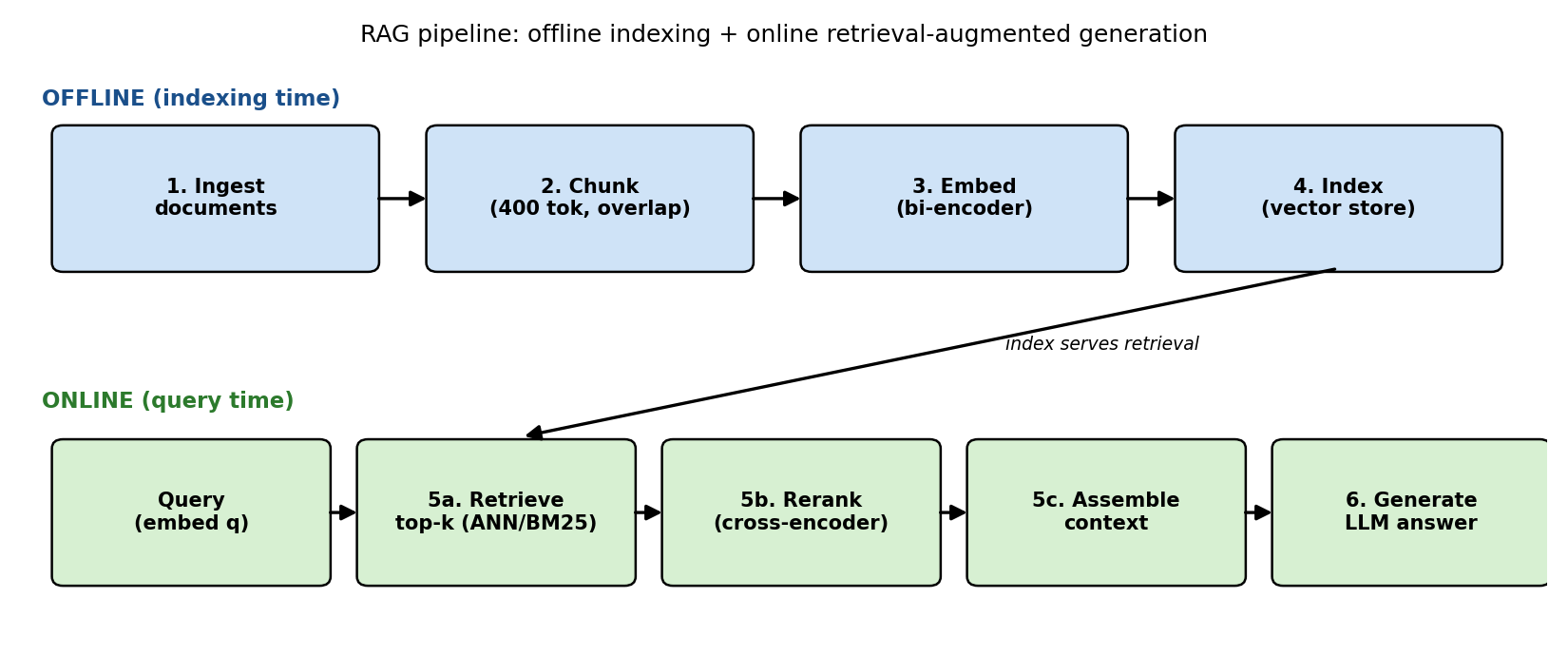
Step	Phase	What happens	Typical tooling
1. Ingest	offline	load documents, clean, extract text	parsers, OCR
2. Chunk	offline	split into retrieval units (200–800 tokens, overlap)	splitter
3. Embed	offline	bi-encoder maps each chunk to a vector	sentence embedder
4. Index	offline	store vectors in a structure that supports fast top-k	vector store
5a. Retrieve	online	embed the query with the same model, search top-k	approximate nearest-neighbour search and/or Best Match 25
5b. Rerank	online (optional)	cross-encoder re-orders the candidates	reranker
5c. Assemble	online	select, truncate, order chunks under the token budget	prompt builder
6. Generate	online	autoregressive decoding conditioned on the context	the language model

Two phases matter for cost analysis: the offline phase is paid once per corpus (and again on updates); the online phase is paid on every query. Anything you can move offline (chunk embeddings, index construction) amortizes; anything online (query embedding, search, reranking, generation) adds to per-query latency.

Knowledge is explicit at inference time (visible chunks you can cite and audit), not implicit in the weights.

Trace of one query through the pipeline

Concrete walkthrough you can reproduce in an exam answer:

1. Offline, done earlier: 1,000 documents → 12,000 chunks of 400 tokens → 12,000 embeddings of dimension 768 → indexed.
2. User asks: "What is the default value of the fusion constant in Reciprocal Rank Fusion?"
3. Embed query with the same bi-encoder used for the chunks (a different model would place the query in an incompatible vector space — classic failure).
4. Retrieve: approximate nearest-neighbour search returns the top 50 chunks by cosine; Best Match 25 returns its own top 50; the lists are fused.
5. Rerank: the cross-encoder scores all fused candidates against the query; keep the best 5.
6. Assemble: 5 × 400 = 2,000 context tokens + instructions + question ≈ 2,500 prompt tokens; best chunk placed first; each chunk tagged [source: doc_017, sec 3].
7. Generate: the model answers "k = 60" and cites doc_017. If the context had not contained the fact, the instructed behaviour is to answer "not found in the provided documents" — refusal is a valid grounded answer.

বাংলা ব্যাখ্যা: পাইপলাইনটা দুই ভাগে ভাবো — অফলাইন অংশে ডকুমেন্ট একবার কেটে, এমবেড করে, ইনডেক্সে রাখা হয়; অনলাইন অংশে প্রতিটি প্রশ্নের জন্য খোঁজা, সাজানো, আর উত্তর তৈরি হয়। খরচের হিসাবে এই ভাগটাই আসল: অফলাইন খরচ একবারই, অনলাইন খরচ প্রতি প্রশ্নে। আর ফর্মুলায় শুধু \(D\) যোগ হয়েছে — ট্রান্সফরমারের ভেতরে কিছুই বদলায়নি, এটা পরীক্ষায় প্রিয় একটা পয়েন্ট। কোয়েরি আর চাঙ্ক একই এমবেডার দিয়ে এমবেড করতে হবে — ভিন্ন মডেল মানেই ভিন্ন ভেক্টর-জগৎ, খোঁজ ব্যর্থ।

End-to-end mini implementation

import numpy as np

docs = [
    "Byte pair encoding is a sub-word tokenization algorithm.",
    "Rotary position embedding rotates query and key vectors.",
    "Reinforcement learning from human feedback trains a reward model.",
]
def embed(text):                       # stand-in embedder
    rng = np.random.default_rng(abs(hash(text)) % (2**32))
    return rng.normal(size=8)

E = np.array([embed(d) for d in docs])           # offline: steps 1-4

def retrieve(q, k=2):                            # online: step 5a
    qe = embed(q)
    sims = E @ qe / (np.linalg.norm(E, axis=1) * np.linalg.norm(qe))
    return [docs[i] for i in np.argsort(-sims)[:k]]

def rag(q):                                      # steps 5c + 6
    ctx = "\n".join(retrieve(q))
    return f"PROMPT: Use only the context.\n{ctx}\nQ: {q}\nA:"

---

4.2 Embedding Models and Chunking

Bi-encoder vs. cross-encoder

• Bi-encoder (dual tower): query and chunk are encoded independently into vectors; similarity is computed afterwards (cosine or dot product). Because the two sides never see each other inside the model, all chunk vectors can be precomputed offline and indexed. Cheap per query, slightly coarse.
• Cross-encoder: one transformer reads the concatenated pair (query, chunk) and outputs a relevance score. Attention flows between query tokens and chunk tokens, so it captures fine interactions (negation, exact constraints). But the score depends on the pair, so nothing can be precomputed — used only for reranking small candidate sets (Section 4.5).

A better embedding model directly raises Recall@k: if the relevant chunk is embedded far from the query, no index or reranker downstream can save you.

Cosine similarity — symbols and worked example (sample-exam topic)

\[\cos(u, v) = \frac{u \cdot v}{\lVert u \rVert \, \lVert v \rVert}\]

Symbol	Meaning
\(u \cdot v\)	dot product \(\sum_i u_i v_i\)
\(\lVert u \rVert\)	Euclidean norm \(\sqrt{\sum_i u_i^2}\)
range	\([-1, 1]\); for non-negative vectors \([0, 1]\)

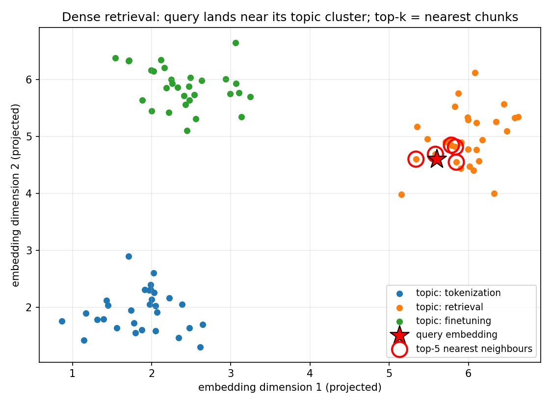
Cosine measures the angle between vectors and ignores their length — two texts about the same topic point in the same direction even if one is longer.

Worked example. Query embedding \(q = (2, 1, 0)\) and three chunk embeddings:

\[d_1 = (1, 1, 0), \qquad d_2 = (0, 1, 1), \qquad d_3 = (2, 0, 1)\]

Norms first: \(\lVert q \rVert = \sqrt{4+1+0} = \sqrt{5} \approx 2.24\); \(\lVert d_1 \rVert = \sqrt{2} \approx 1.41\); \(\lVert d_2 \rVert = \sqrt{2} \approx 1.41\); \(\lVert d_3 \rVert = \sqrt{5} \approx 2.24\).

Chunk	Dot product \(q \cdot d_i\)	Denominator \(\lVert q \rVert \lVert d_i \rVert\)	Cosine	Rank
\(d_1\)	\(2 \cdot 1 + 1 \cdot 1 + 0 = 3\)	\(2.24 \times 1.41 = 3.16\)	\(3 / 3.16 = \mathbf{0.95}\)	1
\(d_2\)	\(0 + 1 + 0 = 1\)	\(2.24 \times 1.41 = 3.16\)	\(1 / 3.16 = \mathbf{0.32}\)	3
\(d_3\)	\(4 + 0 + 0 = 4\)	\(2.24 \times 2.24 = 5.00\)	\(4 / 5.00 = \mathbf{0.80}\)	2

Final retrieval ranking: \(d_1 \;(0.95) \succ d_3 \;(0.80) \succ d_2 \;(0.32)\).

Note the trap: \(d_3\) has the largest dot product (4 > 3) but \(d_1\) has the largest cosine — normalization changes the ranking. This is exactly why you must normalize embeddings (or use unit vectors) before cosine retrieval.

বাংলা ব্যাখ্যা: কোসাইন মাপে দুই ভেক্টরের মধ্যকার কোণ — দৈর্ঘ্য নয়। তাই উপরের উদাহরণে \(d_3\)-এর ডট প্রোডাক্ট বড় হলেও কোসাইনে \(d_1\) জিতেছে, কারণ ভাগ করার সময় ভেক্টরের দৈর্ঘ্য বাদ পড়ে যায়। পরীক্ষায় এই ফাঁদটাই দেওয়া হয়: ডট প্রোডাক্ট দেখে র‍্যাঙ্ক করলে ভুল, নর্ম দিয়ে ভাগ করার পরের মানে র‍্যাঙ্ক করতে হবে। তিন ধাপ মনে রাখো: ডট → নর্মের গুণফল → ভাগ, তারপর সাজাও।

Chunking and context segmentation

Hard rules from the lecture:

• Too short → a chunk loses its surrounding context, becomes ambiguous ("It increased by 12%" — what did?).
• Too long → a chunk mixes topics; the embedding becomes a blurry average and retrieval precision drops; it also wastes the generator's token budget.
• Typical: 200–800 tokens with 10–20% overlap so that facts straddling a boundary survive in at least one chunk.
• Strategies: fixed-size windows, sentence-boundary splitting, recursive splitting on structure (headings → paragraphs → sentences), and per-slide / per-section chunking when documents have natural units.

Chunk-count arithmetic (worked)

With document length \(L\) tokens, chunk size \(C\), overlap \(O\), the window advances by the stride \(S = C - O\) each step. The number of chunks is

\[n_{\text{chunks}} = \left\lceil \frac{L - C}{C - O} \right\rceil + 1\]

Worked example: \(L = 2000\), \(C = 400\), \(O = 100 \Rightarrow S = 300\).

\[n = \left\lceil \frac{2000 - 400}{300} \right\rceil + 1 = \lceil 5.33 \rceil + 1 = 6 + 1 = \mathbf{7 \text{ chunks}}\]

Check by listing start positions: 0, 300, 600, 900, 1200, 1500, 1800 — seven windows; the last covers tokens 1800–2000 (truncated). Storage effect: 7 × 400 = 2800 chunk-tokens for a 2000-token document — overlap costs about 40% extra embedding and storage here.

def chunk(tokens, size=400, overlap=100):
    out, i, step = [], 0, size - overlap
    while i < len(tokens):
        out.append(tokens[i:i + size])
        i += step
    return out

বাংলা ব্যাখ্যা: চাঙ্ক খুব ছোট হলে প্রসঙ্গ হারায়, খুব বড় হলে অনেক বিষয় মিশে এমবেডিং ঝাপসা হয়ে যায় — তাই মাঝামাঝি (২০০–৮০০ টোকেন) রাখা হয়, আর সীমানায় তথ্য যেন না কাটা পড়ে সেজন্য ওভারল্যাপ। সংখ্যা বের করার সূত্রটা সহজ: জানালা প্রতিবার এগোয় (চাঙ্ক − ওভারল্যাপ) ধাপে, তাই \(\lceil (L-C)/(C-O) \rceil + 1\)। পরীক্ষায় সিলিং (উপরের দিকে রাউন্ড) করতে ভুলো না।

---

4.3 Vector Stores and Index Structures

A vector store indexes embeddings for fast top-k lookup. Four index families appear in the lecture; the recurring theme is the speed ↔ recall ↔ memory triangle.

Flat (brute force) — exact, worked cost

Compare the query against every stored vector: per query roughly \(N \cdot d\) multiply–add operations, i.e. about \(2 N d\) floating-point operations, plus the final top-k selection. Complexity \(O(N \cdot d)\).

Worked example: \(N = 1{,}000{,}000\) chunks, \(d = 768\).

• Operations per query: \(2 \times 10^6 \times 768 = 1.54 \times 10^9\) floating-point operations.
• On hardware sustaining \(10^{10}\) operations/second: \(1.54 \times 10^9 / 10^{10} \approx \mathbf{0.15\ s}\) per query — too slow for interactive search, and it scales linearly with \(N\).
• Memory at 32-bit floats: \(10^6 \times 768 \times 4\ \text{B} = \mathbf{3.07\ GB}\).

Flat search is still the right choice for small corpora (up to roughly \(10^5\) vectors) because it is exact (Recall = 1.00) and has zero build cost.

Inverted file index — cluster then probe (worked trade-off)

Build: cluster all vectors into nlist cells (k-means centroids). Search: compare the query to the nlist centroids, then scan only the nprobe closest cells.

Worked example: \(N = 1{,}000{,}000\), nlist \(= 1024\), nprobe \(= 8\).

• Expected vectors scanned: \(N \cdot \frac{nprobe}{nlist} = 10^6 \times \frac{8}{1024} \approx 7813\).
• Total distance computations: \(1024 \text{ (centroids)} + 7813 = 8837\) — about \(\mathbf{113\times}\) fewer than flat search.
• The catch: if the true nearest neighbour sits in a cell that was not probed, it is silently missed → recall < 1.00. Raising nprobe raises recall and cost simultaneously; nprobe = nlist degenerates to flat search.

Hierarchical Navigable Small World — graph index

A multi-layer proximity graph: sparse upper layers for long hops, dense bottom layer for precision. Search descends greedily from the top layer. Expected query complexity \(O(\log N)\) — for \(N = 10^6\), \(\log_2 N \approx 19.93 \approx 20\) greedy descents, a few thousand distance evaluations in total, typically ~1 ms. Build is more expensive, \(O(N \log N)\), and the graph adds memory for the edges, but it supports incremental inserts and gives high recall at high speed — the production default beyond ~\(10^5\) vectors.

Product quantization — compression (worked)

Split each \(d\)-dimensional vector into \(m\) subvectors of \(d/m\) dimensions; quantize each subvector to its nearest centroid out of \(2^{\text{bits}}\) (a codebook learned per subspace); store only the centroid indices.

Worked example: \(d = 128\), \(m = 8\) subvectors, 8 bits per subvector.

• Each subvector of \(128/8 = 16\) dimensions is replaced by one byte (an index into 256 centroids).
• Compressed size: \(m \times 1\ \text{B} = \mathbf{8\ B}\) per vector.
• Uncompressed 32-bit floats: \(128 \times 4 = \mathbf{512\ B}\) per vector.
• Compression ratio: \(512 / 8 = \mathbf{64\times}\).
• At 100 million vectors: \(51.20\ \text{GB} \rightarrow 0.80\ \text{GB}\) — the index now fits in memory.

Price paid: distances are computed between approximations, so ranking quality (recall) degrades slightly; often combined with an inverted file (IVF-PQ) and a re-scoring pass on exact vectors.

Tuning knobs you should be able to name

Index	Parameter	Effect when increased
Inverted file	nlist (number of clusters)	finer partition; cheaper scans per cell but more centroid comparisons; needs more training data
Inverted file	nprobe (cells searched)	recall ↑, latency ↑; nprobe = nlist = flat search
Graph index	M (edges per node)	recall ↑, memory ↑, build time ↑
Graph index	efConstruction	build-time candidate-list size: graph quality ↑, build time ↑
Graph index	efSearch	query-time candidate-list size: recall ↑, latency ↑
Product quantization	\(m\), bits per code	finer codes: accuracy ↑, compression ↓

Every knob trades the same three currencies: speed, recall, memory. An exam answer that names the knob and the currency it spends gets the point.

Comparison table (memorize)

Index	Search complexity	Exact?	Memory	Use when
Flat	\(O(N \cdot d)\)	yes	full vectors	\(N \lesssim 10^5\), need exactness
Inverted file	\(O((nlist + N \cdot \frac{nprobe}{nlist}) \cdot d)\)	no	full vectors + centroids	mid-size, tunable speed/recall
Hierarchical Navigable Small World	\(\approx O(\log N \cdot d)\)	no	vectors + graph edges	large \(N\), low latency, frequent inserts
Product quantization	sub-linear with codes	no	bytes per vector	memory-bound, \(N \gtrsim 10^8\)

বাংলা ব্যাখ্যা: চারটা ইনডেক্স আসলে একই প্রশ্নের চার উত্তর: "সব ভেক্টর না দেখে কীভাবে কাছেরটা পাব?" Flat সব দেখে — নির্ভুল কিন্তু ধীর। Inverted file আগে ক্লাস্টারে ভাগ করে, তারপর কাছের কয়েকটা ক্লাস্টারই দেখে — দ্রুত, কিন্তু ভুল ক্লাস্টারে থাকা সঠিক উত্তর হারিয়ে যেতে পারে। গ্রাফ-ইনডেক্স লগারিদমিক ধাপে নেমে আসে — বড় কর্পাসের ডিফল্ট। আর product quantization ভেক্টরকেই সংকুচিত করে ৬৪ গুণ ছোট করে — মেমরি বাঁচে, নির্ভুলতা একটু কমে। গতি–রিকল–মেমরি, এই তিনের টানাটানিই পুরো গল্প।

---

4.4 Retrieval Mechanisms — Sparse, Dense, Hybrid

Sparse retrieval: Best Match 25 — full formula

\[\text{BM25}(q, d) = \sum_{t \in q} \text{IDF}(t) \cdot \frac{f(t,d)\,(k_1 + 1)}{f(t,d) + k_1\left(1 - b + b \cdot \frac{|d|}{\text{avgdl}}\right)}\]

\[\text{IDF}(t) = \ln\!\left(\frac{N - n(t) + 0.5}{n(t) + 0.5}\right)\]

Symbol	Meaning	Typical value
\(f(t,d)\)	frequency of term \(t\) in document \(d\)	—
$	d	$
avgdl	average document length in the corpus	—
\(N\)	total number of documents	—
\(n(t)\)	number of documents containing \(t\)	—
\(k_1\)	term-frequency saturation parameter	1.5 (range 1.2–2.0)
\(b\)	strength of length normalization	0.75
\(+0.5\)	smoothing in the inverse document frequency	fixed

Three mechanisms to be able to explain:

1. Inverse document frequency with +0.5 smoothing: rare terms (small \(n(t)\)) get large weight; the \(+0.5\) terms prevent division by zero and infinite weights for unseen terms.
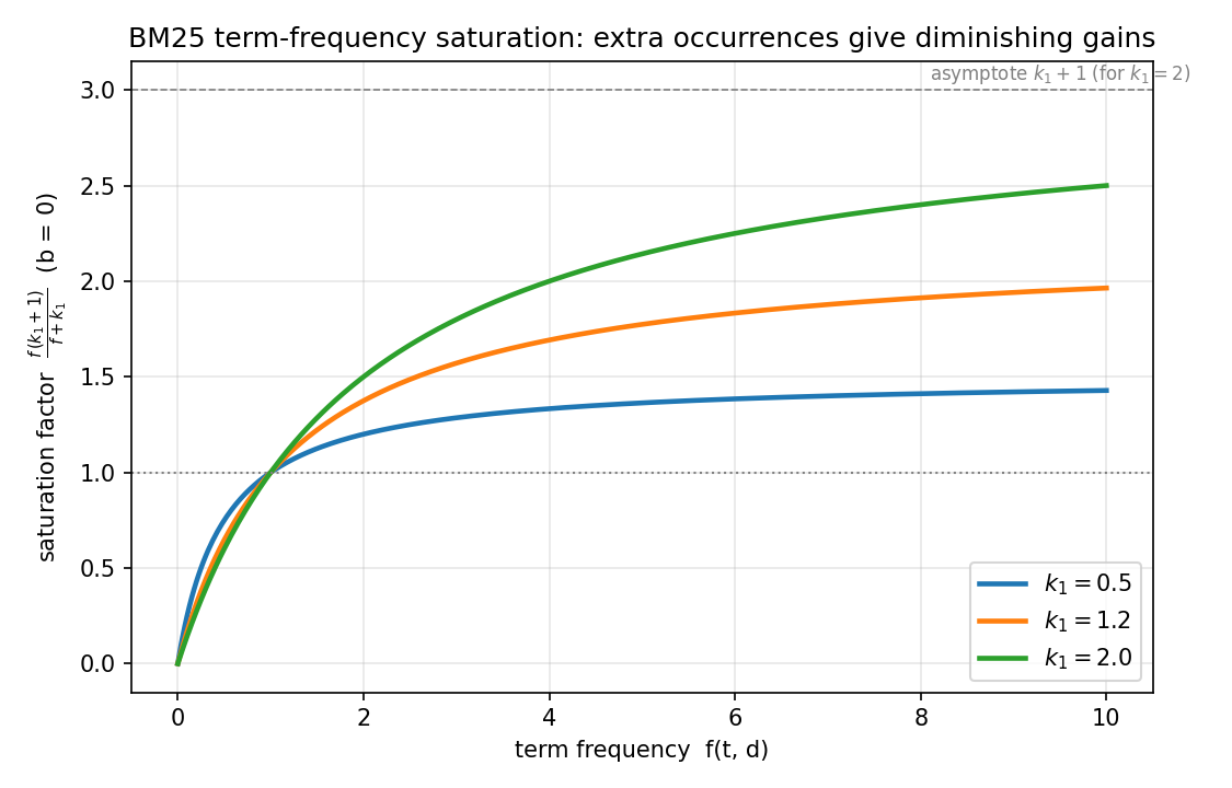
2. Saturation via \(k_1\): the factor \(\frac{f(k_1+1)}{f+k_1}\) grows with \(f\) but is bounded by \(k_1 + 1\) — the 10th occurrence of a term adds far less than the 1st. Small \(k_1\) → saturates almost immediately (near-binary matching); large \(k_1\) → closer to raw term frequency.
3. Length normalization via \(b\): documents longer than average get their effective term frequency discounted (\(b = 1\): full normalization; \(b = 0\): none), so long documents cannot win just by containing more words.

Best Match 25 worked end-to-end (toy corpus)

Corpus (\(N = 3\)), query = "neural retrieval", parameters \(k_1 = 1.5\), \(b = 0.75\):

| Doc | Text | \(|d|\) | \(f(\text{neural}, d)\) | \(f(\text{retrieval}, d)\) | |---|---|---|---|---| | \(D_1\) | "neural networks learn neural representations" | 5 | 2 | 0 | | \(D_2\) | "sparse retrieval ranks documents" | 4 | 0 | 1 | | \(D_3\) | "dense vectors encode semantic meaning" | 5 | 0 | 0 |

Step 1 — corpus statistics. \(\text{avgdl} = (5 + 4 + 5)/3 = 14/3 = 4.67\). Both query terms appear in exactly one document each: \(n(\text{neural}) = 1\), \(n(\text{retrieval}) = 1\).

Step 2 — inverse document frequency (same for both terms).

\[\text{IDF} = \ln\frac{3 - 1 + 0.5}{1 + 0.5} = \ln\frac{2.5}{1.5} = \ln(1.67) = 0.51\]

Step 3 — score \(D_1\) (only "neural" matches, \(f = 2\), \(|d| = 5\)):

• Length ratio: \(|d|/\text{avgdl} = 5/4.67 = 1.07\).
• Denominator add-on: \(k_1 (1 - b + b \cdot 1.07) = 1.5 \times (0.25 + 0.75 \times 1.07) = 1.5 \times 1.05 = 1.58\).
• Saturation fraction: \(\frac{2 \times (1.5 + 1)}{2 + 1.58} = \frac{5.00}{3.58} = 1.40\).
• Score: \(0.51 \times 1.40 = \mathbf{0.71}\).

Step 4 — score \(D_2\) (only "retrieval" matches, \(f = 1\), \(|d| = 4\)):

• Length ratio: \(4/4.67 = 0.86\) (shorter than average → mild boost).
• Denominator add-on: \(1.5 \times (0.25 + 0.75 \times 0.86) = 1.5 \times 0.89 = 1.34\).
• Saturation fraction: \(\frac{1 \times 2.5}{1 + 1.34} = \frac{2.5}{2.34} = 1.07\).
• Score: \(0.51 \times 1.07 = \mathbf{0.55}\).

Step 5 — score \(D_3\): no query term occurs, \(f = 0\) for both → \(\text{BM25}(q, D_3) = \mathbf{0.00}\).

Final ranking: \(D_1\ (0.71) \succ D_2\ (0.55) \succ D_3\ (0.00)\).

Saturation check: if \(D_1\) contained "neural" only once (\(f = 1\)), its score would be \(0.51 \times \frac{2.5}{1 + 1.58} = 0.51 \times 0.97 = 0.49\). Doubling the term frequency raised the score from 0.49 to 0.71 — a factor of 1.45, not 2.00. That is \(k_1\)-saturation in action.

import math
def bm25(query, docs, k1=1.5, b=0.75):
    toks = [d.lower().split() for d in docs]
    N, avg = len(toks), sum(map(len, toks)) / len(toks)
    scores = []
    for d in toks:
        s = 0.0
        for t in query.lower().split():
            f   = d.count(t)
            n_t = sum(1 for dd in toks if t in dd)
            idf = math.log((N - n_t + 0.5) / (n_t + 0.5))
            s  += idf * f * (k1 + 1) / (f + k1 * (1 - b + b * len(d) / avg))
        scores.append(round(s, 2))
    return scores   # [0.71, 0.55, 0.0] for the toy corpus above

বাংলা ব্যাখ্যা: ফর্মুলাটা তিনটা সরল ধারণার গুণফল: (১) বিরল শব্দ বেশি দামি — IDF; (২) একই শব্দ বারবার এলে লাভ কমতে থাকে — \(k_1\) স্যাচুরেশন (১ বার থেকে ২ বারে স্কোর ০.৪৯ → ০.৭১, দ্বিগুণ নয়!); (৩) লম্বা ডকুমেন্ট এমনিতেই বেশি শব্দ ধরে, তাই তাকে ছাড় কম — \(b\) দৈর্ঘ্য-নর্মালাইজেশন। পরীক্ষায় ধাপে ধাপে দেখাও: আগে avgdl আর IDF, তারপর প্রতিটি ডকুমেন্টের ডিনমিনেটর, শেষে গুণ — প্রতিটি সংখ্যা লিখলে আংশিক নম্বরও নিশ্চিত।

How Best Match 25 improves on plain term-frequency–inverse-document-frequency weighting

Aspect	Term-frequency–inverse-document-frequency	Best Match 25
Term frequency	linear (10 occurrences = 10× weight)	saturating, bounded by \(k_1 + 1\)
Document length	optional cosine normalization	explicit, tunable via \(b\) against avgdl
Rare-term weight	\(\log(N / n(t))\)	smoothed \(\ln\frac{N - n(t) + 0.5}{n(t) + 0.5}\)
Tunability	none	\(k_1\) (saturation), \(b\) (length)

Same family of ideas — Best Match 25 is the probabilistically motivated, tunable refinement, and the default lexical baseline to this day.

Dense retrieval

Embed query and chunks with the bi-encoder; rank by cosine (Section 4.2). Strengths: paraphrases ("car" ≈ "automobile"), cross-lingual matching, conceptual similarity. Weakness: rare exact tokens (product codes, error identifiers, names) get smoothed into the surrounding semantics — the embedding has no dedicated dimension for "XJ-4711".

Query type	Sparse (Best Match 25)	Dense (bi-encoder)
"error code XJ-4711"	wins (exact rare token)	often misses
"how do I make my model stop inventing facts"	misses (no term overlap with "hallucination")	wins (semantic match)
cross-lingual question, English corpus	fails (no shared tokens)	wins (shared embedding space)
legal clause with exact citation "§ 433"	wins	risky

Hybrid retrieval and Reciprocal Rank Fusion (worked)

Sparse and dense fail on different queries, so combine them. Score scales are incomparable (Best Match 25 scores vs. cosines), so fuse ranks, not scores:

\[\text{RRF}(d) = \sum_{\text{lists } l} \frac{1}{k + \text{rank}_l(d)}, \qquad k = 60 \text{ (default)}\]

The constant \(k\) damps the influence of top ranks (without it, rank 1 would dominate everything); documents missing from a list simply contribute nothing from that list.

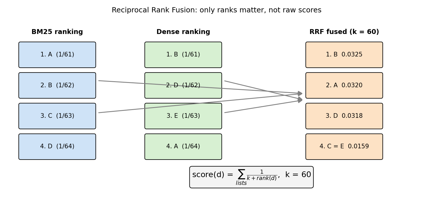
Worked example, \(k = 60\), two ranked lists:

• Best Match 25 ranking: \(A, B, C, D\)
• Dense ranking: \(B, D, E, A\)

Doc	Sparse rank → term	Dense rank → term	RRF score	Final rank
A	1 → \(1/61 = 0.0164\)	4 → \(1/64 = 0.0156\)	\(0.0164 + 0.0156 = \mathbf{0.0320}\)	2
B	2 → \(1/62 = 0.0161\)	1 → \(1/61 = 0.0164\)	\(0.0161 + 0.0164 = \mathbf{0.0325}\)	1
C	3 → \(1/63 = 0.0159\)	—	\(\mathbf{0.0159}\)	4 (tie)
D	4 → \(1/64 = 0.0156\)	2 → \(1/62 = 0.0161\)	\(0.0156 + 0.0161 = \mathbf{0.0318}\)	3
E	—	3 → \(1/63 = 0.0159\)	\(\mathbf{0.0159}\)	4 (tie)

Fused ranking: \(B \succ A \succ D \succ C = E\). Document \(B\) wins because it is good in both lists, even though it tops only one. (The individual scores differ only in the third or fourth decimal place — keep 4 decimals during the computation, then round the final comparison.)

Key property for the exam: Reciprocal Rank Fusion uses only ranks, so it is invariant to any monotone transformation of the underlying scores — no score calibration between sparse and dense systems is needed.

Alternative: weighted score fusion. \(\text{score}(d) = \alpha \cdot \tilde{s}_{\text{dense}}(d) + (1 - \alpha) \cdot \tilde{s}_{\text{sparse}}(d)\) on normalized scores (e.g. min–max per list). More expressive than rank fusion (it can encode "trust the dense system more", \(\alpha > 0.5\)), but it requires score normalization and an extra hyperparameter to tune — exactly the calibration burden that Reciprocal Rank Fusion avoids. Default engineering advice from the lecture: start with rank fusion; switch to weighted fusion only with evaluation data to tune \(\alpha\) on.

বাংলা ব্যাখ্যা: sparse আর dense-এর স্কোর একেবারে আলাদা এককে (একটা BM25 স্কোর, আরেকটা কোসাইন) — সরাসরি যোগ করা যায় না। তাই স্কোর ফেলে দিয়ে শুধু র‍্যাঙ্ক ব্যবহার করা হয়: প্রতিটি তালিকায় যে যত উপরে, সে তত বেশি \(1/(60+r)\) পায়, তারপর যোগফল। দুই তালিকাতেই মোটামুটি ভালো থাকা ডকুমেন্ট (\(B\)) একটিতে চ্যাম্পিয়ন কিন্তু অন্যটিতে অনুপস্থিত ডকুমেন্টকে হারিয়ে দেয় — এটাই হাইব্রিডের শক্তি।

---

4.5 Reranking and Context Assembly

Two-stage design: recall first, precision second

• Retrieval stage (bi-encoder + index, or Best Match 25): cheap, scans millions of chunks, deliberately tuned for recall — cast a wide net (top 50–100), accept noise.
• Reranking stage (cross-encoder): expensive, sees only the candidates, tuned for precision — re-score each (query, chunk) pair jointly and keep the best 5–10.

A reranker can only reorder the candidate set: it raises precision but can never recover a chunk the retrieval stage missed. Recall is bounded by the retrieval stage.

Bi-encoder vs. cross-encoder cost — worked latency estimate

Assume one transformer forward pass costs \(t_f = 10\) ms and the corpus has \(N = 1{,}000{,}000\) chunks.

Strategy	Online work per query	Latency
Bi-encoder + approximate nearest-neighbour index	1 forward pass (embed query) + index search (~5 ms)	\(10 + 5 = \mathbf{15\ ms}\)
Cross-encoder over the whole corpus	\(N\) forward passes: \(10^6 \times 10\ \text{ms} = 10^4\ \text{s}\)	\(\mathbf{\approx 2.78\ h}\) — infeasible
Two-stage: retrieve top 100, cross-encode 100	\(15\ \text{ms} + 100 \times 10\ \text{ms}\)	\(\mathbf{\approx 1.02\ s}\)
Two-stage: retrieve top 20, cross-encode 20	\(15\ \text{ms} + 20 \times 10\ \text{ms}\)	\(\mathbf{\approx 0.22\ s}\)

Why the asymmetry: the bi-encoder's chunk embeddings are precomputed offline — at query time only the query is embedded and compared via fast vector math. The cross-encoder's score is a function of the pair, so there is nothing to precompute: each candidate costs one fresh forward pass at query time. That is the entire reason rerankers are restricted to small \(k\).

An LLM-as-reranker (prompt a large model to order candidates) is even slower and even more accurate — same trade-off, one step further.

Context assembly under a token budget

Select the top-\(n\) reranked chunks that fit the budget, deduplicate near-copies, and order them deliberately: models attend most to the beginning and end of the prompt ("lost in the middle", bowl-shaped attention) — so place the best chunk first or last, never buried in the middle. Add source identifiers so the answer can cite.

বাংলা ব্যাখ্যা: দুই ধাপের শ্রম-বিভাজনটা মনে রাখো: সস্তা ধাপ (bi-encoder) লাখ লাখ চাঙ্ক থেকে মোটামুটি ১০০টা বাছে — জাল বড় করে ফেলা; দামি ধাপ (cross-encoder) সেই ১০০টা মনোযোগ দিয়ে পড়ে সেরা ৫টা রাখে। cross-encoder আগে থেকে হিসাব করা যায় না, কারণ স্কোরটা প্রশ্ন-চাঙ্ক জোড়ার ফাংশন — প্রশ্ন না আসা পর্যন্ত জোড়াই নেই। আর মনে রেখো: রিরr্যাঙ্কার শুধু সাজায়, রিট্রিভাল যা আনেনি তা ফেরাতে পারে না — recall আগের ধাপেই আটকে যায়।

def two_stage(query, store, cross_encoder, k_retrieve=100, k_final=5):
    candidates = store.search(embed(query), k=k_retrieve)       # recall stage
    scored = [(cross_encoder(query, c), c) for c in candidates] # precision stage
    return [c for _, c in sorted(scored, reverse=True)[:k_final]]

---

4.6 Query Decomposition

Hard questions often need evidence that no single chunk contains. Decompose:

• Decompose-then-retrieve: split "Who supervised the doctoral thesis of the founder of company X?" into (1) "Who founded company X?" → answer \(P\); (2) "Who supervised the doctoral thesis of \(P\)?" Retrieve separately, then combine.
• Retrieve–decompose–retrieve loops: the answer to sub-question 1 parameterizes sub-question 2, so retrieval must be interleaved with generation — a first step towards agentic behaviour (Chapter 5).

Related query transformations: query expansion (add synonyms), query rewriting (turn conversational follow-ups into standalone queries — "what about its latency?" → "what is the latency of the Hierarchical Navigable Small World index?").

def multi_hop(question, llm, retrieve):
    subqs = llm(f"Split into sequential sub-questions: {question}")
    notes = []
    for sq in subqs:
        sq_filled = llm(f"Fill placeholders using notes {notes}: {sq}")
        notes.append((sq_filled, retrieve(sq_filled)))
    return llm(f"Answer {question} using {notes}")

বাংলা ব্যাখ্যা: এক চাঙ্কে পুরো উত্তর নেই — এমন প্রশ্নে সরাসরি খোঁজ ব্যর্থ হয়, কারণ প্রশ্নের এমবেডিং দুটি আলাদা তথ্যের মাঝামাঝি কোথাও পড়ে। সমাধান: প্রশ্ন ভেঙে ধাপে ধাপে খোঁজা, যেখানে আগের ধাপের উত্তর পরের ধাপের প্রশ্ন তৈরি করে। এই "খোঁজ → ভাবো → আবার খোঁজ" চক্রই পরের অধ্যায়ের এজেন্টের বীজ।

---

4.7 Evaluating Retrieval-Augmented Generation

Evaluate the two stages separately: a bad answer can come from bad retrieval or from bad generation, and the fix differs.

Retrieval metrics — all on one toy example

Ground truth: relevant chunks for the query are \(\{d_2, d_5, d_9\}\) (3 relevant in total). System returns top-5: \([\,d_7,\ d_2,\ d_9,\ d_1,\ d_3\,]\).

Recall@k — of all relevant chunks, how many did we surface in the top \(k\)?

\[\text{Recall@}k = \frac{|\,\text{relevant} \cap \text{top-}k\,|}{|\,\text{relevant}\,|}\]

Hits in top-5: \(d_2\) (rank 2) and \(d_9\) (rank 3) → 2 hits; \(d_5\) was missed.

\[\text{Recall@5} = \frac{2}{3} = \mathbf{0.67} \qquad \text{Recall@3} = \frac{2}{3} = \mathbf{0.67} \qquad \text{Recall@1} = \frac{0}{3} = \mathbf{0.00}\]

Precision@k — of the \(k\) returned, how many are relevant?

\[\text{Precision@}k = \frac{|\,\text{relevant} \cap \text{top-}k\,|}{k}\]

\[\text{Precision@5} = \frac{2}{5} = \mathbf{0.40} \qquad \text{Precision@3} = \frac{2}{3} = \mathbf{0.67}\]

Reciprocal Rank — how high is the first relevant result? First hit is \(d_2\) at rank 2 → \(\text{RR} = 1/2 = \mathbf{0.50}\).

Mean Reciprocal Rank averages this over a query set:

\[\text{MRR} = \frac{1}{|Q|} \sum_{q \in Q} \frac{1}{r_q}\]

If a second query has its first relevant chunk at rank 1 (\(\text{RR} = 1.00\)):

\[\text{MRR} = \frac{0.50 + 1.00}{2} = \mathbf{0.75}\]

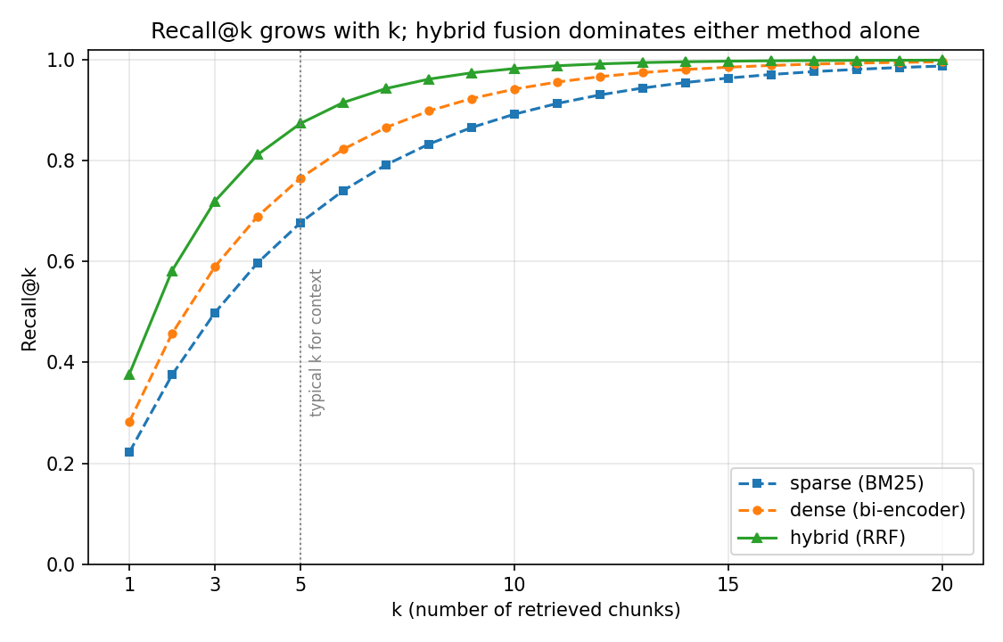
Sanity properties: Recall@k never decreases as \(k\) grows; Precision@k typically decreases as \(k\) grows; Mean Reciprocal Rank only cares about the first hit.

Normalized discounted cumulative gain (mentioned in the lecture, worked briefly). Unlike Recall@k, it rewards placing relevant items higher:

\[\text{DCG@}k = \sum_{i=1}^{k} \frac{\text{rel}_i}{\log_2(i + 1)}, \qquad \text{nDCG@}k = \frac{\text{DCG@}k}{\text{IDCG@}k}\]

For the same toy run, top-3 \(= [d_7, d_2, d_9]\) with binary relevances \((0, 1, 1)\):

• \(\text{DCG@3} = \frac{0}{\log_2 2} + \frac{1}{\log_2 3} + \frac{1}{\log_2 4} = 0 + 0.63 + 0.50 = 1.13\)
• Ideal ordering puts relevant items first: \(\text{IDCG@3} = \frac{1}{1} + \frac{1}{1.58} + \frac{1}{2} = 1 + 0.63 + 0.50 = 2.13\)
• \(\text{nDCG@3} = 1.13 / 2.13 = \mathbf{0.53}\)

Interpretation: the run found two of three relevant chunks (decent recall) but wasted rank 1 on an irrelevant chunk — the position discount cuts the score roughly in half.

Generation metrics

• Faithfulness (groundedness): is every claim in the answer entailed by the retrieved context? Scored 0–1 by a judge model or a natural-language-inference model. Catches the case "retrieval was perfect, the generator hallucinated anyway".
• Answer relevance: does the answer actually address the question (regardless of whether it is grounded)? An answer can be perfectly faithful to the context yet off-topic — and a direct, on-topic answer can be unfaithful.
• Context precision / context relevance: how much of the retrieved context was actually useful — measures retrieval noise reaching the generator.
• Frameworks: RAGAS, ARES, TruLens; failure modes: empty retrieval, irrelevant retrieval, faithfulness failure, citation drift.

Crucial distinction: faithfulness ≠ factual correctness. Faithfulness compares answer ↔ context. If the context itself is wrong or outdated, a perfectly faithful answer is still factually wrong. Factuality needs trusted corpora or external checks.

def recall_at_k(retrieved, relevant, k):
    return len(set(retrieved[:k]) & set(relevant)) / len(relevant)

def mrr(runs):   # runs = list of (retrieved_list, relevant_set)
    total = 0.0
    for retrieved, relevant in runs:
        rr = next((1/r for r, d in enumerate(retrieved, 1) if d in relevant), 0.0)
        total += rr
    return total / len(runs)

বাংলা ব্যাখ্যা: চারটা মেট্রিক চার প্রশ্নের উত্তর: Recall@k — যত প্রাসঙ্গিক চাঙ্ক আছে তার কত ভাগ ধরা পড়ল; Precision@k — যা ধরা পড়ল তার কত ভাগ আসলে কাজের; Mean Reciprocal Rank — প্রথম সঠিকটা কত উপরে; Faithfulness — মডেল কি সত্যিই প্রসঙ্গ থেকে বলছে, নাকি বানাচ্ছে। আর সবচেয়ে সূক্ষ্ম পয়েন্ট: faithful মানেই সঠিক নয় — প্রসঙ্গটা নিজেই ভুল হলে বিশ্বস্ত উত্তরও ভুল। retrieval-এর সমস্যা আর generation-এর সমস্যা আলাদা করে মাপতে হয়, কারণ সমাধানও আলাদা।

---

4.8 Advanced Retrieval-Augmented Generation Architectures

The lecture's framing: a trend of increasing autonomy in the retrieval loop.

1. Hypothetical Document Embeddings: queries and answers live in different "registers" — a short question embeds far from the long factual passage that answers it. Trick: let the model write a hypothetical answer first, embed that, and retrieve with it. The hypothetical answer may be factually wrong; it only has to be stylistically and semantically shaped like the target passage.

def hyde(query, llm, embed, store):
    hypothetical = llm(f"Write a plausible paragraph answering: {query}")
    return store.search(embed(hypothetical), k=5)

1. Self-querying / query rewriting: the model reformulates the user's query (adds filters, resolves pronouns, extracts metadata constraints like year > 2023) before retrieval.
2. Agentic / multi-step retrieval: the model decides what to retrieve, whether the evidence suffices, and when to retrieve again or stop — retrieval becomes a tool in a loop (Chapter 5). Cost: multiple model calls per question, unbounded latency.
3. Graph-based retrieval (Graph-RAG): offline, extract entities and relations into a knowledge graph (often with community summaries). Online, retrieve connected subgraphs instead of isolated chunks. Wins on multi-hop questions whose evidence is spread over documents that share entities but not vocabulary — similarity search cannot jump between them, graph traversal can.
4. Hierarchical retrieval: index summaries of sections/documents; first retrieve at the summary level, then drill down to the chunks beneath the winning summaries. Helps very large or very structured corpora (e.g. legal codes).

বাংলা ব্যাখ্যা: সাধারণ পাইপলাইন এক রাউন্ডে খোঁজে — প্রশ্ন জটিল হলে সেটাই দুর্বলতা। উন্নত রূপগুলোতে মডেল নিজেই খোঁজার প্রক্রিয়ায় হাত দেয়: HyDE-তে আগে কাল্পনিক উত্তর লিখে সেটা দিয়ে খোঁজে (ভুল হলেও আকৃতিটা ঠিক থাকলেই কাজ হয়), agentic সংস্করণে মডেল ঠিক করে আর কত রাউন্ড খুঁজবে, আর graph সংস্করণে ডকুমেন্টের বদলে সম্পর্কের জাল ধরে হাঁটা যায় — বহু-ধাপ প্রশ্নে যেটা অপরিহার্য। স্বাধীনতা যত বাড়ে, ক্ষমতা তত বাড়ে — সাথে খরচ আর লেটেন্সিও।

---

4.9 Retrieval Latency, Cost, and System Considerations

The latency budget

End-to-end latency = embed query + search index + rerank + assemble + generate. Typical shape:

Stage	Typical latency	Scales with
Query embedding	5–20 ms	model size
Index search	1–50 ms	\(N\), index type, nprobe / ef parameters
Cross-encoder rerank	100–1000 ms	\(k \times\) forward-pass time
Generation	1–10 s	output length × time per token (+ prefill ∝ context length)

Generation usually dominates — but note that stuffing more chunks into the prompt increases prefill time and cost, so retrieval quality (fewer, better chunks) directly buys generation speed.

Worked budget. Query embedding 10 ms + graph-index search 5 ms + cross-encoder rerank of 20 candidates at 10 ms each = 200 ms + generation of 300 output tokens at 20 ms/token = 6,000 ms. Total \(\approx 10 + 5 + 200 + 6000 = \mathbf{6{,}215\ ms}\), of which generation is \(6000 / 6215 = \mathbf{96.54\%}\). Lesson: optimizing the index from 5 ms to 1 ms is invisible; trimming the context (faster prefill) or streaming tokens to the user changes perceived latency far more.

Retrieval vs. long context — cost per query (worked)

Corpus: a 250,000-token manual. Model price: $3.00 per million input tokens.

• Long-context approach (paste the whole manual every time): \(250{,}000 \times \$3.00 / 10^6 = \mathbf{\$0.75}\) per query — plus a very long prefill.
• Retrieval approach (top-5 chunks × 400 tokens + ~500 tokens of prompt and question ≈ 2,500 tokens): \(2{,}500 \times \$3.00 / 10^6 = \mathbf{\$0.0075}\) per query.
• Ratio: \(0.75 / 0.0075 = \mathbf{100\times}\) cheaper per query, before caching.

Long context still wins when the corpus is small, every part of it matters (whole-document summarization, contract comparison), or engineering an index is not worth it. Retrieval wins on large corpora, high query volume, and freshness.

Keeping the index fresh

• Full rebuild: re-chunk, re-embed, re-index everything. Simple, consistent, expensive — fine nightly for small corpora.
• Incremental upsert: insert/update/delete individual chunk vectors (graph indexes support inserts well; deletions often become tombstones that degrade the structure until a periodic rebuild).
• Delta index: new documents go into a small fresh index searched alongside the main one; merge periodically.
• Consistency trade-off: between update and re-index, queries may retrieve stale or deleted content — the answer cites a document version that no longer exists. Mitigations: timestamp metadata filters, versioned indexes with atomic swap.
• Remember the dual cost of any document change: the embedding compute and the index maintenance.

Caching

Cache (query → retrieved set) for popular queries, cache embeddings of repeated texts, and use the model provider's prompt caching for the static prompt prefix.

বাংলা ব্যাখ্যা: সিস্টেম-চোখে দেখলে প্রশ্নপ্রতি খরচই আসল: পুরো ম্যানুয়াল প্রতিবার পাঠালে $০.৭৫, আর খুঁজে এনে দরকারি ২,৫০০ টোকেন পাঠালে $০.০০৭৫ — একশো গুণ সস্তা। কিন্তু ফ্রি লাঞ্চ নেই: ইনডেক্স বানাতে ও তাজা রাখতে হয়, আর আপডেটের ফাঁকে পুরনো/মুছে-ফেলা তথ্য উঠে আসার ঝুঁকি (staleness) থাকে। rebuild সহজ-কিন্তু-দামি, upsert সস্তা-কিন্তু-অগোছালো — এই টানাটানিই মিনি-কেস প্রশ্নের প্রিয় বিষয়।

---

Derivations and Proof Sketches (TU-hard corner)

Where the Best Match 25 inverse document frequency comes from

The binary independence model scores a document by the log-odds that its terms appear in relevant vs. non-relevant documents:

\[w(t) = \log \frac{p(t \mid R)\,\bigl(1 - p(t \mid \bar R)\bigr)}{p(t \mid \bar R)\,\bigl(1 - p(t \mid R)\bigr)}\]

With no relevance information, assume \(p(t \mid R) = 0.5\) (the first fraction cancels) and estimate \(p(t \mid \bar R) \approx n(t)/N\) (the term's overall document frequency). Adding \(0.5\) to each count for smoothing (a continuity correction that keeps the estimate finite when \(n(t) = 0\) or \(n(t) = N\)) gives

\[w(t) = \log \frac{N - n(t) + 0.5}{n(t) + 0.5}\]

— exactly the inverse-document-frequency factor of Best Match 25. Note it goes negative when \(n(t) > N/2\): a term in more than half the documents is evidence against relevance; many implementations clamp it at zero or add \(+1\) inside the logarithm.

Why Reciprocal Rank Fusion is invariant to monotone score transformations

Let \(f\) be strictly increasing and let \(s_l(d)\) be the scores in list \(l\). Ranks are defined by comparisons: \(\text{rank}_l(d) < \text{rank}_l(d')\) iff \(s_l(d) > s_l(d')\). Applying \(f\) preserves every comparison (\(f(s) > f(s') \iff s > s'\)), hence preserves every rank, hence preserves every term \(1/(k + \text{rank}_l(d))\) and the fused ordering. Consequence: the sparse system can report scores in \([0, 25]\) and the dense system cosines in \([-1, 1]\) — fusion is unaffected, which is precisely why no calibration step is needed.

Why reranking cannot raise recall (one-line proof)

Let \(C\) be the candidate set returned by retrieval and \(R\) the relevant set. The reranker outputs a permutation of \(C\), so its output set is still \(C\); hence \(|R \cap C|\) — the numerator of recall — is unchanged by any reranker, while precision at small \(k\) can improve by moving the relevant members of \(C\) to the front.

বাংলা ব্যাখ্যা: তিনটা ছোট প্রমাণ — পরীক্ষার সবচেয়ে কঠিন প্রশ্নগুলো এখান থেকেই আসে। IDF আসলে সম্ভাবনার লগ-অডস থেকে আসা, +0.5 শুধু শূন্য-ভাগ ঠেকানোর স্মুদিং; RRF র‍্যাঙ্ক ছাড়া কিছু দেখে না বলে স্কোরের একক যা-ই হোক ফলাফল একই; আর রিরr্যাঙ্কার যেহেতু শুধু সাজায় — সেট বদলায় না — recall-এর লব অপরিবর্তিত থাকে। যুক্তিগুলো এক লাইনে বলতে পারলেই পূর্ণ নম্বর।

---

Real-World Deployment Patterns and Limitations

Use case	Design choices that matter
Internal documentation question answering	small corpus → flat or graph index; hybrid retrieval; nightly re-index
Customer support assistant	frequently-asked-questions + tickets + product docs; reranker is critical (noisy corpus); strict citation format
Legal contract assistant	long structured documents → hierarchical retrieval; citations mandatory; staleness guarantees (Section 4.9)
Coding assistant	code-aware chunking (functions/classes as units); small fast embedding model; exact-identifier queries favour sparse retrieval
Web-search answer summaries	web-scale index; freshness pipeline; aggressive caching
Compliance and audit	faithfulness checks on every answer; trusted-source filtering; versioned indexes

Hard limitations to state in mini-cases:

1. Retrieval-Augmented Generation cannot answer what is not in the corpus — it relocates the knowledge problem, it does not solve coverage.
2. Prompt injection via documents: a retrieved chunk may contain adversarial instructions ("ignore your previous instructions and …"); the generator reads it as context with near-instruction authority. Mitigations: treat retrieved text as data (delimiters, instruction hierarchy), sanitize corpora, restrict tool use (Chapters 5 and 7).
3. Latency stack-up: every added stage (rerank, multi-hop, agentic loops) multiplies per-query latency.
4. Garbage in, garbage out: contradictory or outdated documents produce faithful-but-wrong answers; corpus curation is part of the system.

Choosing between retrieval, finetuning, and long context

Criterion	Retrieval-Augmented Generation	Finetuning (Chapter 6)	Long context
Knowledge freshness	re-index — minutes	retrain — days	paste latest — instant
Private/dynamic facts	excellent	poor (bakes in a snapshot)	good for small corpora
Style/format/behaviour change	weak	excellent	weak
Per-query cost	low (small context)	lowest (no context)	highest
Traceability/citations	natural	none	possible but unaided
Upfront engineering	index + evaluation pipeline	training pipeline + data	none

Rule of thumb from the lecture: knowledge → retrieval; behaviour → finetuning; small static corpus + global tasks → long context. They compose: a finetuned model can sit inside a retrieval pipeline.

বাংলা ব্যাখ্যা: মিনি-কেস প্রশ্নে এই টেবিলটাই তোমার অস্ত্র: প্রশ্নে "জ্ঞান বদলায়" শুনলেই retrieval, "ভঙ্গি/ফরম্যাট বদলাও" শুনলেই finetuning, "ছোট কর্পাস, পুরোটা একসাথে দেখতে হবে" শুনলেই long context। আর সীমাবদ্ধতার তালিকা থেকে অন্তত একটা trade-off উল্লেখ করতে ভুলো না — কৌশল + যুক্তি + trade-off, এই তিনে পাঁচ নম্বর।

---

Exam-Focused Summary

Topic	Memorize
Conditional language modelling	\(P(y \mid q, D) = \prod_t P(y_t \mid y_{<t}, q, D)\)
Six-step pipeline	ingest → chunk → embed → index ‖ retrieve → rerank → assemble → generate
Cosine	\(\frac{u \cdot v}{\lVert u \rVert \lVert v \rVert}\); normalize first; angle not length
Best Match 25	inverse document frequency (+0.5 smoothing) × saturation (\(k_1\)) × length norm (\(b\))
Reciprocal Rank Fusion	\(\sum_l 1/(k + \text{rank}_l)\), \(k = 60\); ranks only, monotone-invariant
Index types	flat \(O(Nd)\) exact; inverted file nlist/nprobe; graph \(O(\log N)\); product quantization 64× compression
Chunk count	\(\lceil (L - C)/(C - O) \rceil + 1\)
Bi vs. cross encoder	precompute offline vs. \(N\) forward passes per query
Retrieval metrics	Recall@k, Precision@k, Mean Reciprocal Rank
Generation metrics	faithfulness (answer ↔ context), answer relevance (answer ↔ question)
Reranking bound	raises precision, can never raise recall

Common traps:

1. Ranking by dot product when the question asks for cosine — normalize first.
2. Forgetting the \(+1\) in the chunk-count formula, or forgetting to take the ceiling.
3. Confusing Recall@k (denominator = number of relevant) with Precision@k (denominator = \(k\)).
4. Claiming a reranker improves recall — it cannot; it only reorders.
5. Treating faithfulness as factual correctness — context itself can be wrong.
6. Adding raw Best Match 25 scores to cosine scores instead of fusing ranks.
7. Believing retrieval eliminates hallucination — it only reduces it.
8. Ignoring prompt injection through retrieved documents (a document can carry adversarial instructions).

বাংলা ব্যাখ্যা: রিভিশনের সময় এই টেবিলটা দিয়ে নিজেকে কুইজ করো: প্রতিটি সারির ডান কলাম ঢেকে রেখে বাঁ কলাম দেখে ফর্মুলা/বাক্যটা বলতে পারো কি না। ফাঁদের তালিকাটা আরও দামি — পরীক্ষার ভুলের ৮০% এই আট লাইনের মধ্যেই থাকে।

Thirty-second flashcards

• Q: What does Retrieval-Augmented Generation change in the model? — A: Nothing in the weights; only the conditioning set: \(P(y \mid q, D)\).
• Q: Two reasons to chunk with overlap? — A: Facts straddling a boundary survive; chunks keep local context.
• Q: Why normalize before cosine? — A: Cosine compares angles; unnormalized dot products favour long vectors and can change the ranking.
• Q: What bounds the Best Match 25 saturation factor? — A: \(k_1 + 1\).
• Q: What does \(b = 0\) mean? — A: No length normalization; \(b = 1\) is full normalization.
• Q: Why \(+0.5\) in the inverse document frequency? — A: Smoothing — avoids division by zero and unbounded weights for terms in zero or all documents.
• Q: Inverted file index misses a neighbour — when? — A: When the true neighbour lies in a cell not among the nprobe probed cells.
• Q: Product quantization with \(d = 128\), \(m = 8\), 8 bits — bytes per vector? — A: 8 bytes vs. 512 bytes uncompressed, \(64\times\).
• Q: Why can a reranker never raise recall? — A: It only reorders the retrieved candidate set; missed chunks stay missed.
• Q: Reciprocal Rank Fusion constant and default? — A: \(k\) in \(1/(k + \text{rank})\), default 60; damps the dominance of rank 1.
• Q: Faithfulness vs. answer relevance? — A: Answer ↔ context entailment vs. answer ↔ question pertinence.
• Q: Recall@k as \(k \to\) corpus size? — A: Tends to 1.00; precision tends to (number relevant)/\(N\).
• Q: When does long context beat retrieval? — A: Small corpus, global tasks (summarize everything), low query volume.
• Q: Hypothetical Document Embeddings in one line? — A: Embed a generated hypothetical answer instead of the query; shape matters, truth does not.

---

Mock Exam — Chapter 4

Time guide: ~45 minutes for this chapter's share. Use the technical terms from the lecture. Do not use abbreviations. Round numerical results to 2 decimal places unless asked otherwise. A non-programmable calculator is allowed.

Level 1 — Basic (multiple choice and definitions)

Q1.1 (1 pt). Which statement best describes what Retrieval-Augmented Generation changes about a pretrained language model?

• (a) It updates the model weights with new documents at inference time.
• (b) It conditions the unchanged generator on retrieved external context at inference time.
• (c) It replaces autoregressive decoding with nearest-neighbour lookup of answers.
• (d) It compresses the document collection into the model's weights.

Q1.2 (1 pt). Which statement best describes the difference between a bi-encoder and a cross-encoder?

• (a) The bi-encoder scores the query–document pair jointly; the cross-encoder encodes them independently.
• (b) The bi-encoder encodes query and document independently so document vectors can be precomputed; the cross-encoder reads the pair jointly and must run one forward pass per pair at query time.
• (c) Both can precompute document representations; the cross-encoder is simply larger.
• (d) The cross-encoder is used for indexing and the bi-encoder for reranking.

Q1.3 (1 pt). Which index structure always returns the exact nearest neighbours?

• (a) Inverted file index with nprobe < nlist.
• (b) Hierarchical Navigable Small World graph.
• (c) Flat (brute-force) index.
• (d) Product quantization codes.

Q1.4 (1 pt). Which statement about Reciprocal Rank Fusion is correct?

• (a) It requires calibrating the sparse and dense scores to a common scale.
• (b) It uses only the rank positions, so any monotone transformation of the underlying scores leaves the fused ranking unchanged.
• (c) It weights each list by its raw score variance.
• (d) It can only fuse exactly two ranked lists.

Q1.5 (2 pts). Define faithfulness of a generated answer in a Retrieval-Augmented Generation system, and state how it differs from factual correctness.

Q1.6 (2 pts). Define Recall@k with its formula and state what happens to it as \(k\) increases.

Level 2 — Intuitive ("Explain why …", 3 pts each: cause → mechanism → consequence)

Q2.1. Explain why hybrid retrieval outperforms purely dense retrieval on queries containing rare exact terms such as product codes or error identifiers.

Q2.2. Explain why the retrieval stage is tuned for recall while the reranking stage is tuned for precision, and not the other way around.

Q2.3. Explain why cross-encoder relevance scores cannot be precomputed offline the way bi-encoder document embeddings can.

Level 3 — Harder (numerical, 5 pts each, show every step)

Q3.1 (Recall and Mean Reciprocal Rank). A test set has two queries. Query 1: relevant chunks \(\{a, c\}\); system returns \([\,b, a, d, c, e\,]\). Query 2: relevant chunk \(\{f\}\); system returns \([\,f, g, h, i, j\,]\). (a) Compute Recall@3 for each query. (b) Compute the Reciprocal Rank for each query and the Mean Reciprocal Rank over the test set.

Q3.2 (Best Match 25). Corpus statistics: \(N = 10\) documents, the query consists of the single term "tensor" with \(n(\text{tensor}) = 2\), average document length \(\text{avgdl} = 60\). Parameters \(k_1 = 1.2\), \(b = 0.75\). Document \(A\): \(f = 3\), \(|d| = 90\). Document \(B\): \(f = 1\), \(|d| = 30\). Compute both scores (2 decimals), give the ranking, and explain why tripling the term frequency did not triple the score.

Q3.3 (Fusion and compression). (a) Fuse with Reciprocal Rank Fusion (\(k = 60\)): sparse list \([X, Y, Z]\), dense list \([Y, Z, W]\). Give all scores to 4 decimal places and the final ranking. (b) A store holds 10 million vectors with \(d = 768\) in 32-bit floats. Compute the memory footprint, then the footprint under product quantization with \(m = 96\) subvectors at 8 bits each, and the compression ratio.

Level 4 — Transfer (TU-hard, 5 pts each)

Q4.1 (Retrieval vs. long context). A support team answers 10,000 queries per month against a 250,000-token product manual. Input tokens cost $3.00 per million. Compare the monthly input-token cost of (i) pasting the full manual into every prompt and (ii) a retrieval pipeline that sends 2,500 tokens per query. Then name two situations in which the long-context approach is still the better engineering choice.

Q4.2 (Graph-based retrieval). "Which professor supervised the doctoral thesis of the founder of the company that acquired DeepStart?" — explain why a standard similarity-based pipeline fails on this question and how graph-based retrieval addresses it. Name one cost of the graph approach.

Q4.3 (Index staleness mini-case). A legal-tech firm updates 2% of its 5-million-chunk corpus daily; answers must never cite withdrawn documents. Propose an indexing/update strategy (technique + justification + trade-off).

Level 5 — Coding (worked solutions below; outputs verified by execution)

Q5.1. Implement cosine top-k retrieval with NumPy over a toy corpus of 5 chunk embeddings and evaluate Recall@2 and Mean Reciprocal Rank for two queries with known relevant sets.

Q5.2. Implement Reciprocal Rank Fusion (\(k = 60\)) merging a sparse ranking and a dense ranking, and print the fused scores.

---

Solutions

Level 1

A1.1 — (b). The transformer and its weights are untouched; only the conditioning set changes: \(P(y \mid q, D)\) instead of \(P(y \mid q)\). (a) describes finetuning; (c) abolishes generation; (d) describes pretraining.

A1.2 — (b). Independence of the two towers is exactly what makes offline precomputation and indexing possible; joint attention over the pair is what makes the cross-encoder accurate and non-precomputable. (a) swaps the definitions; (c) is false for the cross-encoder; (d) reverses the pipeline roles.

A1.3 — (c). Flat search compares the query with every vector — exact by construction, cost \(O(N \cdot d)\). The inverted file index can miss neighbours in unprobed cells; the graph index is greedy and approximate; product quantization compares compressed approximations.

A1.4 — (b). \(\text{score}(d) = \sum_l 1/(k + \text{rank}_l(d))\) consumes ranks only. Monotone transformations of scores preserve order, hence ranks, hence the fused result. (a) is the problem Reciprocal Rank Fusion avoids; (d) it generalizes to any number of lists.

A1.5. Faithfulness is the degree (0–1) to which every claim in the generated answer is entailed by the retrieved context — the answer asserts nothing the context does not support. It differs from factual correctness because the comparison target is the context, not the world: if the retrieved context itself is wrong or outdated, a perfectly faithful answer is still factually wrong.

A1.6. \(\text{Recall@}k = \frac{|\text{relevant} \cap \text{top-}k|}{|\text{relevant}|}\) — the fraction of all relevant chunks that appear among the \(k\) retrieved. It is monotonically non-decreasing in \(k\): enlarging the retrieved set can only add hits, never remove them (at $k = $ corpus size, Recall = 1.00).

Level 2

A2.1. Cause: dense embedding models compress text into a few hundred dimensions trained on general semantic similarity; a rare token such as "XJ-4711" contributes almost nothing distinctive to the vector — it is smoothed into the surrounding semantics. Mechanism: sparse retrieval (Best Match 25) scores by exact term overlap weighted by inverse document frequency, and a term occurring in very few documents receives a very large weight, so the one chunk containing the code dominates the sparse ranking; hybrid fusion (Reciprocal Rank Fusion) lets that sparse signal reach the final list even when the dense list misses it. Consequence: the hybrid system retrieves the correct chunk for identifier-style queries while keeping dense retrieval's strength on paraphrases — higher recall across both query types than either method alone.

A2.2. Cause: the two stages face different candidate-set sizes and cost constraints — the first stage must scan millions of chunks cheaply, the second sees only dozens. Mechanism: any relevant chunk dropped by the first stage is unrecoverable, because the reranker can only reorder what it is given — recall is bounded by retrieval; conversely, false positives from the first stage can still be removed later by the precise (but expensive) cross-encoder. Consequence: errors of omission are fatal in stage one but errors of inclusion are not, so the cheap stage casts a wide, noisy net (high recall, top 50–100) and the expensive stage filters it (high precision, top 5). Reversing the tuning would either miss evidence permanently or make the pipeline computationally infeasible.

A2.3. Cause: a cross-encoder's relevance score is a function of the pair — query tokens and document tokens attend to each other inside one forward pass. Mechanism: before the query arrives, the pair does not exist; there is no query-independent intermediate representation that could be stored, unlike the bi-encoder, whose document tower runs without the query and whose vectors can be indexed offline. Consequence: every candidate costs one fresh forward pass at query time — \(O(k)\) passes per query — which is why cross-encoders are applied only to small reranking sets (e.g. 20–100 candidates ≈ 0.2–1.0 s) and never to the full corpus (\(10^6\) passes ≈ 2.78 hours per query).

Level 3

A3.1. (a) Query 1, top-3 \(= [b, a, d]\): hits \(= \{a\}\), so \(\text{Recall@3} = 1/2 = \mathbf{0.50}\). Query 2, top-3 \(= [f, g, h]\): hits \(= \{f\}\), so \(\text{Recall@3} = 1/1 = \mathbf{1.00}\). (b) Query 1: first relevant is \(a\) at rank 2 → \(\text{RR}_1 = 1/2 = 0.50\). Query 2: first relevant is \(f\) at rank 1 → \(\text{RR}_2 = 1.00\).

\[\text{MRR} = \frac{0.50 + 1.00}{2} = \mathbf{0.75}\]

A3.2. Inverse document frequency (one term, shared by both documents):

\[\text{IDF} = \ln\frac{N - n + 0.5}{n + 0.5} = \ln\frac{10 - 2 + 0.5}{2 + 0.5} = \ln\frac{8.5}{2.5} = \ln(3.40) = 1.22\]

Document \(A\) (\(f = 3\), \(|d| = 90\)): length ratio \(90/60 = 1.50\); denominator add-on \(k_1(1 - b + b \cdot 1.50) = 1.2 \times (0.25 + 1.125) = 1.2 \times 1.375 = 1.65\); saturation fraction \(\frac{3 \times 2.2}{3 + 1.65} = \frac{6.6}{4.65} = 1.42\); score \(= 1.22 \times 1.42 = \mathbf{1.74}\).

Document \(B\) (\(f = 1\), \(|d| = 30\)): length ratio \(30/60 = 0.50\); add-on \(1.2 \times (0.25 + 0.375) = 0.75\); fraction \(\frac{1 \times 2.2}{1 + 0.75} = \frac{2.2}{1.75} = 1.26\); score \(= 1.22 \times 1.26 = \mathbf{1.54}\).

Ranking: \(A\ (1.74) \succ B\ (1.54)\). Although \(A\) has three times the term frequency, its score is only \(1.74/1.54 = 1.13\times\) higher: the saturation factor is bounded by \(k_1 + 1 = 2.2\), so repeated occurrences add diminishing value, and \(A\) is additionally penalized for being longer than average (\(b\)-length normalization) while \(B\) is boosted for being shorter.

A3.3. (a) Contributions: rank 1 → \(1/61 = 0.0164\), rank 2 → \(1/62 = 0.0161\), rank 3 → \(1/63 = 0.0159\).

Doc	Sparse	Dense	Total
X	\(0.0164\)	—	\(\mathbf{0.0164}\)
Y	\(0.0161\)	\(0.0164\)	\(\mathbf{0.0325}\)
Z	\(0.0159\)	\(0.0161\)	\(\mathbf{0.0320}\)
W	—	\(0.0159\)	\(\mathbf{0.0159}\)

Fused ranking: \(Y \succ Z \succ X \succ W\). The two documents present in both lists beat the single-list winners.

(b) Uncompressed: \(10^7 \times 768 \times 4\ \text{B} = 10^7 \times 3072\ \text{B} = \mathbf{30.72\ GB}\). Product quantization: \(m = 96\) codes × 1 byte = 96 B per vector → \(10^7 \times 96\ \text{B} = \mathbf{0.96\ GB}\). Compression ratio: \(3072 / 96 = \mathbf{32\times}\) (each 8-dimensional subvector of 32-bit floats, 32 B, becomes one byte). Trade-off: distances are computed on approximations, so recall drops slightly; usually mitigated by re-scoring the top candidates with exact vectors.

Level 4

A4.1. (i) Full manual: \(250{,}000\) tokens × $3.00/10^6 = $0.75 per query; monthly: \(10{,}000 \times 0.75 = \mathbf{\$7{,}500.00}\). (ii) Retrieval: \(2{,}500 \times 3.00/10^6 = \$0.0075\) per query; monthly: \(10{,}000 \times 0.0075 = \mathbf{\$75.00}\). Saving: \(7{,}500 - 75 = \$7{,}425.00\) per month — a \(100\times\) ratio (ignoring the comparatively small one-time embedding/indexing cost and the retrieval infrastructure). Long context still wins when: (1) the task needs global views of the document — whole-manual summarization, cross-section consistency checks — where retrieval's isolated chunks lose information; (2) the corpus is small, the query volume is low, or provider-side prompt caching makes repeated context cheap, so the engineering and maintenance cost of a retrieval pipeline (chunking, index freshness, evaluation) is not justified. (Also acceptable: prototyping, or when retrieval quality on the domain is known to be poor.)

A4.2. Why similarity search fails: the question requires a chain of facts — acquirer of DeepStart → founder of that acquirer → thesis supervisor of that founder — that no single chunk contains; the question's embedding is not close to any one passage, and the intermediate entities (the acquirer, the founder) are not even named in the query, so single-shot nearest-neighbour retrieval has nothing to anchor on. How graph-based retrieval fixes it: offline, entities (companies, people) and relations (acquired, founded by, supervised by) are extracted into a knowledge graph; at query time, retrieval traverses edges — DeepStart →(acquired by)→ Company → (founded by) → Person → (supervised by) → Professor — pulling the connected subgraph (or its community summary) into the context, so the generator sees the complete chain. Cost: expensive offline construction (entity/relation extraction over the whole corpus, typically with a language model) plus extraction errors that propagate into answers, and graph maintenance on every corpus update.

A4.3. Technique: incremental updates with a delta index plus tombstoning and metadata filtering: new and revised chunks are upserted into a small fresh index that is searched alongside the main Hierarchical Navigable Small World index; withdrawn documents are immediately marked with tombstones / a validity flag, and the retrieval layer applies a mandatory metadata filter (status = active) so deleted content can never be returned even before physical removal; the delta index is merged into the main index in a periodic (e.g. nightly) rebuild with atomic index swap. Justification: 2% of 5 million chunks = 100,000 chunks/day — a daily full re-embed and rebuild of all 5 million is wasteful, while pure in-place deletion in a graph index degrades its structure; the filter, not the index structure, carries the hard legal guarantee "never cite withdrawn documents", which makes correctness independent of rebuild timing. Trade-off: two indexes must be queried and their results fused (extra latency and operational complexity), tombstones accumulate and reduce index efficiency until the merge, and between upserts the freshest documents may rank slightly worse in the small delta index (consistency vs. cost: full rebuilds give a perfectly consistent snapshot but at much higher compute).

Level 5

A5.1 — cosine top-k retrieval + evaluation (executed; output below).

import numpy as np

E = np.array([
    [0.9, 0.1, 0.0],   # 0: "BM25 sparse retrieval"
    [0.8, 0.3, 0.1],   # 1: "inverted index term match"
    [0.1, 0.9, 0.2],   # 2: "dense embeddings cosine"
    [0.0, 0.8, 0.4],   # 3: "bi-encoder vector search"
    [0.2, 0.2, 0.9],   # 4: "cross-encoder reranking"
], dtype=float)

queries  = np.array([[0.85, 0.2, 0.05],     # sparse-flavoured query
                     [0.05, 0.85, 0.3]])    # dense-flavoured query
relevant = [{0, 1}, {2, 3}]

def top_k(q, E, k):
    En = E / np.linalg.norm(E, axis=1, keepdims=True)   # normalize rows
    qn = q / np.linalg.norm(q)                          # normalize query
    sims = En @ qn                                      # cosine = dot of unit vectors
    order = np.argsort(-sims)[:k]
    return order.tolist(), sims[order].round(2).tolist()

def recall_at_k(ranked, rel, k):
    return len(set(ranked[:k]) & rel) / len(rel)

def mrr(all_ranked, all_rel):
    rr = []
    for ranked, rel in zip(all_ranked, all_rel):
        rr.append(next((1.0 / r for r, d in enumerate(ranked, 1) if d in rel), 0.0))
    return sum(rr) / len(rr)

ranked_lists = []
for i, q in enumerate(queries):
    ranked, sims = top_k(q, E, k=5)
    ranked_lists.append(ranked)
    print(f"query {i}: ranking {ranked}  sims {sims}")
    print(f"  Recall@2 = {recall_at_k(ranked, relevant[i], 2):.2f}")
print(f"MRR = {mrr(ranked_lists, relevant):.2f}")

Verified output:

query 0: ranking [0, 1, 2, 4, 3]  sims [0.99, 0.99, 0.34, 0.31, 0.23]
  Recall@2 = 1.00
query 1: ranking [2, 3, 4, 1, 0]  sims [0.99, 0.99, 0.53, 0.42, 0.16]
  Recall@2 = 1.00
MRR = 1.00

Both queries place a relevant chunk at rank 1 (Reciprocal Rank \(= 1.00\) each), so the Mean Reciprocal Rank is \(1.00\); both relevant chunks per query land in the top 2, so Recall@2 \(= 1.00\). Key implementation points: normalize both matrix rows and query before the dot product (otherwise it is dot-product ranking, not cosine), and use argsort(-sims) for descending order.

A5.2 — Reciprocal Rank Fusion merge (executed; output below).

def rrf_merge(list_a, list_b, k=60):
    scores = {}
    for lst in (list_a, list_b):
        for rank, doc in enumerate(lst, 1):       # ranks start at 1
            scores[doc] = scores.get(doc, 0.0) + 1.0 / (k + rank)
    return sorted(scores.items(), key=lambda kv: -kv[1])

sparse = ["D1", "D4", "D2"]
dense  = ["D3", "D1", "D5"]
for doc, s in rrf_merge(sparse, dense):
    print(f"{doc}: {s:.4f}")

Verified output:

D1: 0.0325
D3: 0.0164
D4: 0.0161
D2: 0.0159
D5: 0.0159

D1 wins because it appears in both lists (\(1/61 + 1/62 = 0.0325\)); every other document appears in only one list and contributes a single reciprocal term. Note enumerate(lst, 1): starting ranks at 0 is the classic off-by-one bug in Reciprocal Rank Fusion implementations.

বাংলা ব্যাখ্যা: মক পরীক্ষাটা স্তরে স্তরে সাজানো — L1 সংজ্ঞা চেনে কি না, L2 "কেন"-চেইন বানাতে পারো কি না, L3 ক্যালকুলেটরে ধাপে ধাপে সংখ্যা বের করতে পারো কি না, L4 নতুন পরিস্থিতিতে জ্ঞান বসাতে পারো কি না, L5 কোডে নামাতে পারো কি না। আসল পরীক্ষার আগে L3-এর তিনটা অঙ্ক হাতে-কলমে (ক্যালকুলেটর দিয়ে) আবার করো — BM25-এর ধাপগুলো মুখস্থ নয়, অভ্যাস হয়ে যাওয়া চাই।

---

End of Chapter 4.