Chapter 1: Introduction to AI Engineering
Course: AI Engineering, WS 2025/2026 — Dr.-Ing. Johannes Abel, IfN, TU Braunschweig PDF mapped:
AI_Engineering_WS20252026_Ch1.pdf(25 slides) Code mapped:0-1-python-basics.ipynb,0-2-files-and-data.ipynb,0-3-pytorch-intro.ipynb,0-4-pytorch-advanced.ipynb
0. How to Study This Chapter (Exam Format Reminder)
The written exam is 120 minutes, 50 points, answers in English, non-programmable calculator allowed. The official instruction on the cover sheet is: "Use the technical terms from the lecture. Do not use abbreviations." All numerical results must be rounded to 2 decimal places (very small probabilities may be written in scientific notation with a 2-decimal mantissa, e.g. \(3.00 \times 10^{-4}\)).
Question types you must train for:
- Fundamentals: multiple choice with exactly one correct option ("Which statement best describes…").
- Analysis: "Explain why…" questions worth 3 points — structure every answer as cause → mechanism → consequence.
- Application: mini-case questions worth 5 points — name the technique, give a justification, and state one trade-off.
বাংলা ব্যাখ্যা: পরীক্ষায় শুধু সংজ্ঞা মুখস্থ বললে পুরো নম্বর পাওয়া যায় না। "Explain why" প্রশ্নে কারণ → ভেতরের প্রক্রিয়া → ফলাফল — এই তিন ধাপে উত্তর সাজাতে হবে। সংখ্যার উত্তর সবসময় দুই দশমিক ঘর পর্যন্ত লিখবে, আর লেকচারের পারিভাষিক শব্দগুলো (technical terms) পুরো নামসহ ব্যবহার করবে, সংক্ষিপ্ত রূপ নয়।
1. Chapter Overview
This chapter motivates the entire course. It explains why the field of "AI Engineering" emerged, introduces the central technical idea behind modern AI systems (next-word prediction → Large Language Models → Foundation Models), and gives a road map for all later chapters.
Why this chapter matters:
- It sets the vocabulary that the rest of the lecture uses (Large Language Model, Foundation Model, modality, Generative Pretrained Transformer, fine-tuning, Retrieval-Augmented Generation, agent).
- It establishes the engineering perspective: AI Engineering is not about training new models from scratch; it is about building reliable products on top of pre-trained foundation models.
- It ties classical machine-learning ideas (probability theory, sequence modelling) to modern systems (chat assistants, code generation, speech recognition).
Connections:
- Backwards (prerequisites): Pattern Recognition, basic probability theory, basic neural networks.
- Forwards: Chapter 2 explains how Large Language Models are built (the topics named here in 1.2–1.4 in detail). Chapter 3 builds on the chat-style interaction sketched in 1.1. Chapters 4–5 generalize the idea of "foundation model + extra context" (1.4 → Chapter 4) and "foundation model + actions" (1.4 → Chapter 5). Chapters 6–7 cover post-training adaptation and the legal and ethical wrap-up named in 1.6.
High-probability exam topics from this chapter:
- Define a Foundation Model and contrast it with a classical task-specific machine-learning model.
- Explain the next-word prediction problem using a bigram example (with numbers).
- Explain the role of the language model in automatic speech recognition (Bayes decision rule / noisy channel).
- A short numerical exercise: bigram estimation from a toy corpus, sentence probability, possibly perplexity.
- A multiple-choice question on which component of "Chat / Generative / Pretrained / Transformer" names the architecture.
বাংলা ব্যাখ্যা: এই অধ্যায়টা পুরো কোর্সের ভিত্তি। মূল বার্তা একটাই — "পরের শব্দটা অনুমান করো" এই ছোট্ট সমস্যাটাকে বিশাল মাপে নিয়ে গেলেই আজকের ChatGPT-জাতীয় সিস্টেম পাওয়া যায়। আর AI Engineering মানে নিজে মডেল ট্রেইন করা নয়, বরং তৈরি মডেলের ওপর নির্ভরযোগ্য প্রোডাক্ট বানানো।
2. Beginner-Friendly Intuition
Story. Imagine a phone keyboard that suggests the next word as you type. If you type "Good", it might suggest "morning". That tiny prediction trick — given the words so far, predict the most likely next word — is the entire core idea of modern AI. Scale that idea up by a factor of a billion (more data, a bigger network, more compute) and you get ChatGPT.
Real-life analogies.
- A translator who learned by reading. A person who has read millions of books in a hundred languages can do many tasks (translate, summarize, write a poem) just by being asked. They never trained specifically on each task — the knowledge transferred. That is exactly what foundation models do.
- Speech recognition. When you speak into your phone, two systems cooperate: an acoustic model (sound → candidate words) and a language model (which word sequence is linguistically plausible). The language model is doing next-word prediction, constrained by the acoustic evidence.
Why does this field exist? For decades, artificial intelligence tried to hand-engineer every task: a separate spam filter, a separate translator, a separate chatbot. Around 2017–2022 the field discovered that a single model trained on next-word prediction at giant scale becomes competent at all of those tasks — often zero-shot, without any task-specific training. That discovery changed the economics and the engineering practice of the whole industry.
Without this chapter you cannot follow the rest of the course: you would not know what a Large Language Model is, what the foundation-model paradigm promises, why prompts matter at all, or why the lecture spends most of its time on Chapter 2.
বাংলা ব্যাখ্যা: মোবাইলের কীবোর্ড যেমন পরের শব্দ সাজেস্ট করে, আধুনিক AI ঠিক সেই কাজটাই করে — শুধু কোটি কোটি গুণ বড় পরিসরে। আগে প্রতিটা কাজের জন্য আলাদা মডেল বানাতে হতো; এখন একটা বিশাল মডেলই সব কাজ পারে। এই "এক মডেল, অনেক কাজ" ধারণাটাই foundation model-এর মূল কথা।
3. Key Concepts and Definitions (Glossary)
| Term | Meaning | বাংলা | Example |
|---|---|---|---|
| Artificial Intelligence | Computer systems that perform tasks that normally require human intelligence | কম্পিউটার দিয়ে বুদ্ধিমত্তার কাজ করানো | Chess engines, ChatGPT, self-driving cars |
| Machine Learning | Programs that learn patterns from data instead of being hand-coded | নিয়ম হাতে না লিখে ডেটা থেকে প্যাটার্ন শেখা | A spam filter trained on labelled emails |
| Deep Learning | Machine learning with neural networks that have many layers | বহু স্তরের নিউরাল নেটওয়ার্ক দিয়ে শেখা | A 50-layer image classifier |
| Language Model | A model that assigns probabilities to word sequences | শব্দের ধারার সম্ভাবনা হিসাব করার মডেল | \(P(\text{cat} \mid \text{the}) = 0.50\) |
| Bigram | A pair of consecutive tokens; a first-order Markov language model | পাশাপাশি দুটি শব্দ; শুধু আগের শব্দটা দেখে | "the cat", "cat sat" |
| Token | The smallest unit a model reads (word, sub-word, or byte piece) | মডেল যাকে একটি একক হিসেবে পড়ে | "playing" → ["play", "ing"] |
| Vocabulary | The set of all distinct tokens the model knows; size \(V\) | মডেলের চেনা সব টোকেনের তালিকা | \(V = 6\) for the toy corpus below |
| Large Language Model | A language model with billions of parameters trained on web-scale text | বিশাল আকারের সাধারণ-উদ্দেশ্যের ভাষা মডেল | GPT-4, LLaMA-3, Claude, Gemini |
| Transformer | The attention-based neural architecture behind modern language models | আজকের ভাষা মডেলের মূল স্থাপত্য | "Attention is All You Need", 2017 |
| Foundation Model | A model pretrained on broad data that can be adapted to many downstream tasks | এক মডেল, বহু কাজে অভিযোজনযোগ্য | LLaMA-3 used for chat, code, summarization |
| Pretraining | The expensive, large-scale, self-supervised first training stage | বড় পরিসরের প্রাথমিক প্রশিক্ষণ | LLaMA pretraining on roughly 15 trillion tokens |
| Fine-tuning | Comparatively cheap adaptation of a pretrained model to a specific task | নির্দিষ্ট কাজের জন্য ছোট পরিসরের শোধন | Tuning LLaMA for medical question answering |
| Modality | A type of data: text, image, audio, video | ডেটার ধরন: লেখা, ছবি, শব্দ, ভিডিও | Image-text models such as CLIP |
| Generative Model | A model that produces new data rather than only labels | নতুন কনটেন্ট তৈরি করে, শুধু লেবেল দেয় না | DALL-E (images), GPT (text) |
| Autoregressive Generation | Producing output one token at a time, each conditioned on all previous tokens | এক টোকেন করে, আগেরগুলোর ওপর শর্ত রেখে তৈরি | GPT-style decoding |
| Markov Assumption | Approximating the full history by only the last \(n-1\) tokens | পুরো ইতিহাস নয়, শুধু শেষ কয়েকটা শব্দ দেখা | Bigram: only the previous token matters |
| Maximum Likelihood Estimation | Estimating probabilities as relative frequencies from counts | গণনা থেকে আপেক্ষিক হার দিয়ে সম্ভাবনা নির্ণয় | \(\hat P(\text{cat}\mid\text{the}) = C(\text{the cat})/C(\text{the})\) |
| Perplexity | \(P(w_{1..N})^{-1/N}\); the average branching factor of a language model | মডেল গড়ে কতগুলো শব্দের মধ্যে দ্বিধায় থাকে | Lower perplexity = better model |
| Acoustic Model | In speech recognition: models \(P(X \mid W)\), audio given words | শব্দতরঙ্গ আর শব্দের মিল মাপে | Part of the noisy-channel decoder |
| Noisy Channel Model | Decoding rule \(\hat W = \arg\max_W P(X \mid W)\,P(W)\) | শ্রবণ-প্রমাণ ও ভাষাগত স্বাভাবিকতা একসাথে | Automatic speech recognition |
| ChatGPT | The OpenAI chat application built on GPT models | GPT মডেলের ওপর বানানো চ্যাট অ্যাপ্লিকেশন | Released November 30, 2022 |
| AI Engineering | The discipline of building products on top of foundation models | তৈরি মডেল দিয়ে বাস্তব প্রোডাক্ট বানানোর প্রকৌশল | A retrieval-based customer-support bot |
বাংলা ব্যাখ্যা: এই টেবিলের প্রতিটা শব্দ পরীক্ষায় "technical term" হিসেবে ব্যবহার করতে হবে — সংক্ষিপ্ত রূপ নয় (যেমন "LLM" না লিখে "Large Language Model" লিখবে)। সবচেয়ে গুরুত্বপূর্ণ পার্থক্যটা মনে রাখো: Language Model হলো ধারণা, Large Language Model তার বিশাল সংস্করণ, আর Foundation Model হলো আরও বড় ছাতা — যার নিচে টেক্সট ছাড়াও ছবি, অডিও, ভিডিওর মডেলও পড়ে।
4. Section-by-Section Lecture Notes
Section 1.1 — The AI Revolution
What the slides say
- ChatGPT was the trigger event: released November 30, 2022, it reached 100 million users in about 2 months — the fastest consumer-software adoption in history at that time.
- The acronym in "ChatGPT" decomposes as: Chat = the conversational user interface, Generative = the model produces new text, Pretrained = trained beforehand on huge corpora, Transformer = the neural network architecture.
- Success factors listed on the slides: free trial access, conversational user experience, in-session memory, broad domain competence, fluent text generation, social-media virality, post-pandemic timing, mature cloud infrastructure, and integration into products and application programming interfaces.
- News headlines (Nature, The New York Times, Bloomberg) illustrate the cultural shift, not just the technical one.
Beginner explanation
Before ChatGPT, using artificial intelligence required a developer: an application programming interface call, a model setup, some glue code. ChatGPT removed that barrier — anyone with a browser and a question could "use AI". That is what "the AI revolution" refers to in this course.
Technical explanation
The technical foundation is a GPT-3.5-class model refined with reinforcement learning from human feedback (details in Chapter 2). The chat front-end keeps a running context — a prefix containing all previous turns — and sends it to the model on every turn. This gives the user the illusion of memory, but the model itself is stateless: the chat application re-sends the conversation history with every request.
Common mistakes
- Believing ChatGPT "remembers" you across sessions (by default it does not — memory is an application-layer feature).
- Confusing the application (ChatGPT) with the model (GPT-3.5 / GPT-4).
- Saying "Transformer" is the product name — it is the architecture.
Exam relevance
- "Which component of 'Chat Generative Pretrained Transformer' names the architecture?" — guaranteed warm-up multiple-choice material.
- "Name three success factors of ChatGPT" — pick any three from the slide list above.
- "Explain why a chat assistant appears to remember the conversation" — cause: stateless model; mechanism: the application re-sends the full history as context; consequence: apparent memory limited by context length.
বাংলা ব্যাখ্যা: ChatGPT-এর সাফল্যের আসল কারণ প্রযুক্তি যতটা, ততটাই সহজলভ্যতা — ব্রাউজার খুলে প্রশ্ন করলেই উত্তর। আর একটা জরুরি সূক্ষ্মতা: মডেল নিজে কিছুই "মনে রাখে না"; চ্যাট অ্যাপ প্রতিবার পুরনো কথোপকথনটা আবার পাঠায় বলে মনে রাখার ভ্রম তৈরি হয়। পরীক্ষায় এই পয়েন্টটা প্রায়ই আসে।
Minimal code example: a chat loop is string concatenation
# Simulated chat loop. The "model" is faked so the file runs offline.
from typing import List, Dict

def fake_llm(messages: List[Dict[str, str]]) -> str:
    """A pretend language model: returns the last user message reversed."""
    last_user = next(m["content"] for m in reversed(messages) if m["role"] == "user")
    return f"(echo) {last_user[::-1]}"

def chat():
    history = [{"role": "system", "content": "You are a helpful tutor."}]
    user_inputs = ["What is a token?", "Give me one example."]
    for u in user_inputs:
        history.append({"role": "user", "content": u})
        reply = fake_llm(history)          # the WHOLE history is sent every turn
        history.append({"role": "assistant", "content": reply})
        print(f"USER:      {u}")
        print(f"ASSISTANT: {reply}\n")

chat()
Key point: the illusion of memory comes from re-sending history on every call — exactly how real chat application programming interfaces work.
Section 1.2 — The Next-Word Prediction Problem
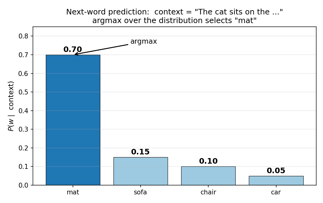
This is the mathematical heart of Chapter 1. Everything later in the course (Transformers, prompting, sampling) refines this one problem.
1.2.1 Language modelling and the chain rule
A language model assigns a probability to a sequence of tokens \(w_1, w_2, \ldots, w_T\). The exact factorization uses the chain rule of probability:
Symbol definitions:
| Symbol | Meaning | Example |
|---|---|---|
| \(w_t\) | the token at position \(t\) | \(w_3 = \text{"AI"}\) in "I love AI" |
| \(T\) | total length of the sequence | \(T = 3\) for "I love AI" |
| \(\prod_{t=1}^{T}\) | product over all positions \(1 \ldots T\) | multiply the per-token probabilities |
| \(P(w_t \mid w_1,\ldots,w_{t-1})\) | conditional probability of the next token given the full history | "given everything so far, how likely is this word?" |
The chain rule is exact — no approximation yet. It only rewrites a joint probability as a product of conditionals. (Derivation: apply the definition of conditional probability \(P(A,B) = P(A)\,P(B \mid A)\) repeatedly.)
Worked numeric example. Sentence: "I love AI", so \(w_1 = \text{I}\), \(w_2 = \text{love}\), \(w_3 = \text{AI}\).
Step by step: (1) write the chain-rule factorization, (2) insert the given conditional probabilities, (3) multiply. Sentence probabilities shrink fast — that is why practical systems work with log probabilities (sums instead of products).
বাংলা ব্যাখ্যা: একটা বাক্যের মোট সম্ভাবনা মানে — প্রতিটা শব্দ তার আগের সব শব্দ দেখে কতটা স্বাভাবিক, সেই শর্তাধীন সম্ভাবনাগুলোর গুণফল। chain rule কোনো অনুমান নয়, এটা সম্ভাবনার একটা নির্ভুল পুনর্লিখন। গুণ করতে করতে সংখ্যা খুব ছোট হয়ে যায় বলে বাস্তবে আমরা logarithm নিয়ে যোগ করি।
1.2.2 The bigram approximation (first-order Markov assumption)
Conditioning on the entire history is impossible for count-based models, so the bigram model keeps only the previous token:
The conditional probabilities are estimated by maximum likelihood estimation — counting:
| Symbol | Meaning |
|---|---|
| \(C(w_{t-1}, w_t)\) | number of times the bigram (pair) occurs in the training corpus |
| \(C(w_{t-1})\) | number of times the previous word occurs in the training corpus |
| \(\hat P\) | an estimated probability (hat = estimate from data) |
Fully worked toy-corpus example. Training corpus (extends the slide example "the cat sat on the mat"):
the cat sat on the mat the cat slept on the mat
Step 1 — tokenize: 12 tokens, vocabulary \(V = 6\) distinct types.
Step 2 — unigram counts:
| Word | \(C(w)\) |
|---|---|
| the | 4 |
| cat | 2 |
| on | 2 |
| mat | 2 |
| sat | 1 |
| slept | 1 |
Step 3 — bigram counts (11 adjacent pairs):
| Bigram | \(C(w_{t-1}, w_t)\) |
|---|---|
| the cat | 2 |
| the mat | 2 |
| on the | 2 |
| cat sat | 1 |
| cat slept | 1 |
| sat on | 1 |
| slept on | 1 |
| mat the | 1 |
Step 4 — bigram probabilities (rounded to 2 decimals):
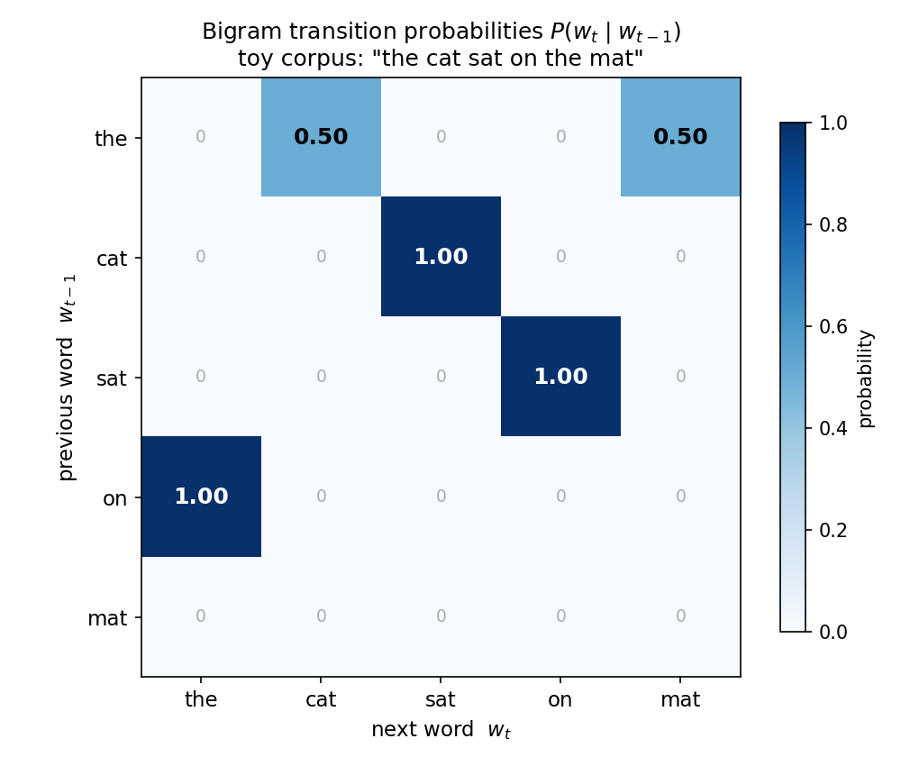
The complete transition table (rows = previous word \(w_{t-1}\), columns = next word \(w_t\); rounded to 2 decimals, dash = zero count):
| \(w_{t-1}\) next: | the | cat | sat | slept | on | mat |
|---|---|---|---|---|---|---|
| the | – | 0.50 | – | – | – | 0.50 |
| cat | – | – | 0.50 | 0.50 | – | – |
| sat | – | – | – | – | 1.00 | – |
| slept | – | – | – | – | 1.00 | – |
| on | 1.00 | – | – | – | – | – |
| mat | 0.50 | – | – | – | – | – |
Reading example: the row "cat" says that after "cat" the model expects "sat" or "slept", each with probability \(0.50\). Every row of a complete transition table must sum to \(1.00\) — a quick sanity check during the exam. (The "mat" row sums to \(0.50\) only because the final corpus token has no successor; see the trap note below.)
Step 5 — probability of a full sentence. For "the cat sat on the mat" (6 tokens), start with the unigram probability of the first word, \(P(\text{the}) = 4/12 \approx 0.33\), then chain the bigrams:
Side note: "the cat slept on the mat" receives exactly the same probability \(1/24 \approx 0.04\), because the model considers "sat" and "slept" equally likely after "cat" — a count-based model cannot prefer one over the other with these data.
Contrast sentence: "the mat sat on the cat" contains the bigram (mat, sat), which never occurs in the corpus, so \(\hat P(\text{sat} \mid \text{mat}) = 0/2 = 0.00\) and the whole sentence probability collapses to 0.00 — even though the sentence is grammatically fine. This is the zero-count problem (picked up again in the mock exam, Level 4).
Log-space version (how it is done in practice). Multiplying many probabilities quickly underflows floating-point arithmetic, so real systems sum base-2 logarithms instead of multiplying probabilities:
| Factor | Probability | \(\log_2\) value |
|---|---|---|
| \(P(\text{the})\) | \(0.33\) | \(-1.58\) |
| \(\hat P(\text{cat} \mid \text{the})\) | \(0.50\) | \(-1.00\) |
| \(\hat P(\text{sat} \mid \text{cat})\) | \(0.50\) | \(-1.00\) |
| \(\hat P(\text{on} \mid \text{sat})\) | \(1.00\) | \(0.00\) |
| \(\hat P(\text{the} \mid \text{on})\) | \(1.00\) | \(0.00\) |
| \(\hat P(\text{mat} \mid \text{the})\) | \(0.50\) | \(-1.00\) |
| Sum | \(-4.58\) |
Check: \(2^{-4.58} \approx 0.04 = 1/24\) — consistent with the direct product. The same value \(-4.58\) reappears in the perplexity computation (1.2.5) and in the verified program output of the mock exam (Level 5). Remember for the exam: a more negative log probability means a less probable sentence.
Exam traps:
- Wrong denominator: divide by the count of the previous word, \(C(w_{t-1})\) — not by the corpus length and not by the vocabulary size.
- Distinguish \(P(w_t)\) (unigram) from \(P(w_t \mid w_{t-1})\) (bigram) — read the question carefully.
- Subtle point: the final corpus token ("mat" at the end) has no successor, so the outgoing probabilities of "mat" sum to \(0.50\), not \(1.00\), under the lecture convention of dividing by the unigram count. Mention this only if asked; for calculations always use the convention above.
বাংলা ব্যাখ্যা: bigram মডেলের পুরো হিসাবটা আসলে গোনাগুনতি — জোড়াটা কতবার এসেছে, ভাগ করো আগের শব্দটা কতবার এসেছে দিয়ে। সবচেয়ে কমন ভুল হলো ভাজক: মোট শব্দসংখ্যা দিয়ে ভাগ নয়, আগের শব্দের সংখ্যা দিয়ে ভাগ। আর যে জোড়া কর্পাসে একবারও আসেনি, তার সম্ভাবনা শূন্য — ফলে পুরো বাক্যের সম্ভাবনাই শূন্য হয়ে যায়, এটাই zero-count সমস্যা।
1.2.3 Why n-gram models break down
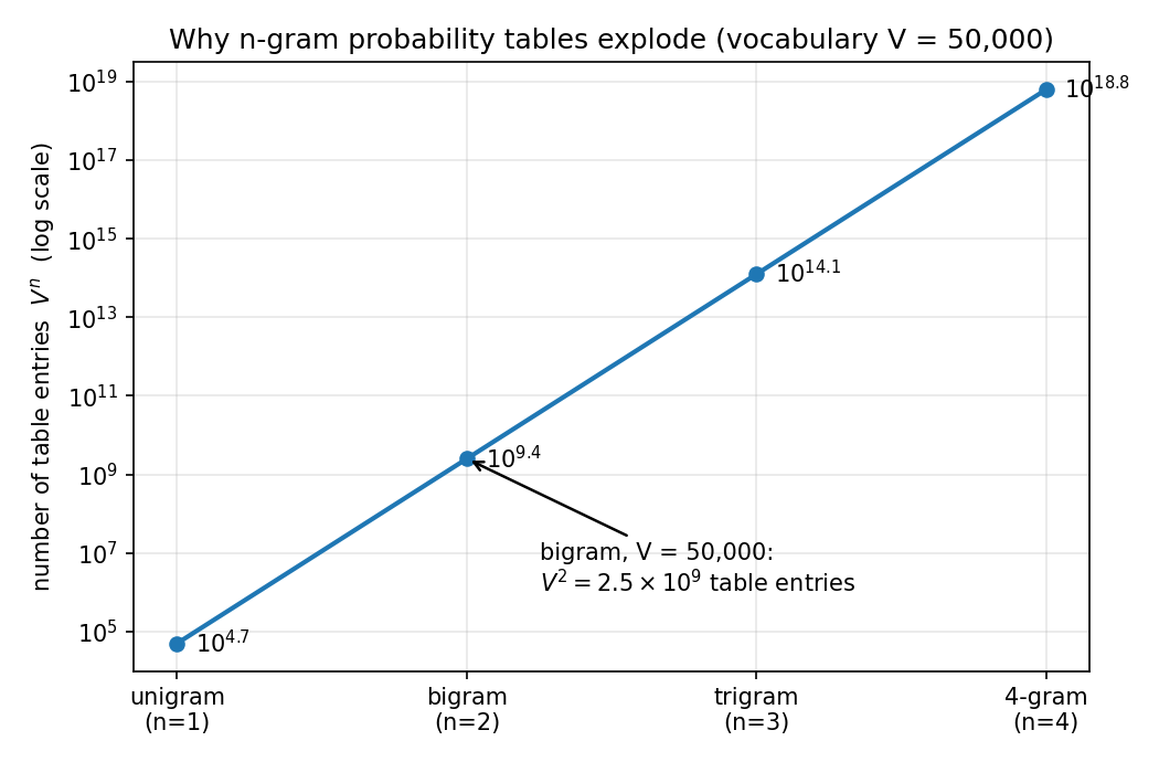
Generalizing to an n-gram model, \(P(w_t \mid w_{t-n+1}, \ldots, w_{t-1})\), looks attractive, but:
- The number of possible n-grams grows as \(V^n\) — for a vocabulary of \(V = 50{,}000\) and \(n = 5\), that is \(50{,}000^5 \approx 3.13 \times 10^{23}\) possible contexts. No corpus on Earth covers a meaningful fraction of them.
- Data sparsity: most grammatical n-grams are never observed → zero counts everywhere.
- The Markov assumption is hard-limited: a 5-gram model can never connect "The girl who grew up in Braunschweig speaks fluent ___" to "German", because the clue lies more than 4 tokens back.
- No generalization across similar words: "the cat sat" and "the dog sat" are unrelated events to a count-based model.
This motivates neural language models — a parametric function \(f_\theta(w_1, \ldots, w_{t-1})\) that outputs a probability distribution over the vocabulary — and ultimately Large Language Models (Section 1.3).
বাংলা ব্যাখ্যা: n বাড়ালে প্রসঙ্গ (context) বড় হয় ঠিকই, কিন্তু সম্ভাব্য n-gram-এর সংখ্যা \(V^n\) হারে বিস্ফোরিত হয় — কোনো কর্পাসেই এত উদাহরণ নেই। তাছাড়া count-ভিত্তিক মডেল "cat" আর "dog"-এর মিল বোঝে না, প্রতিটা জোড়াকে আলাদা ঘটনা ভাবে। এই দুই সীমাবদ্ধতাই নিউরাল ভাষা মডেলের জন্ম দিয়েছে।
1.2.4 The classical application: language models in automatic speech recognition
Automatic speech recognition is the classical motivation for language models. Given acoustic features \(X\) (the audio), find the most probable word sequence \(\hat W\). Apply Bayes' theorem (noisy channel model):
| Symbol | Meaning |
|---|---|
| \(X\) | observed acoustic feature sequence (the audio evidence) |
| \(W\) | a candidate word sequence (hypothesis) |
| \(\hat W\) | the recognized (chosen) word sequence |
| \(P(X \mid W)\) | acoustic model: how well the audio matches the hypothesis |
| \(P(W)\) | language model: prior probability that anyone would say this sequence |
| \(P(X)\) | evidence; constant over all hypotheses \(W\), so it can be dropped from the \(\arg\max\) |
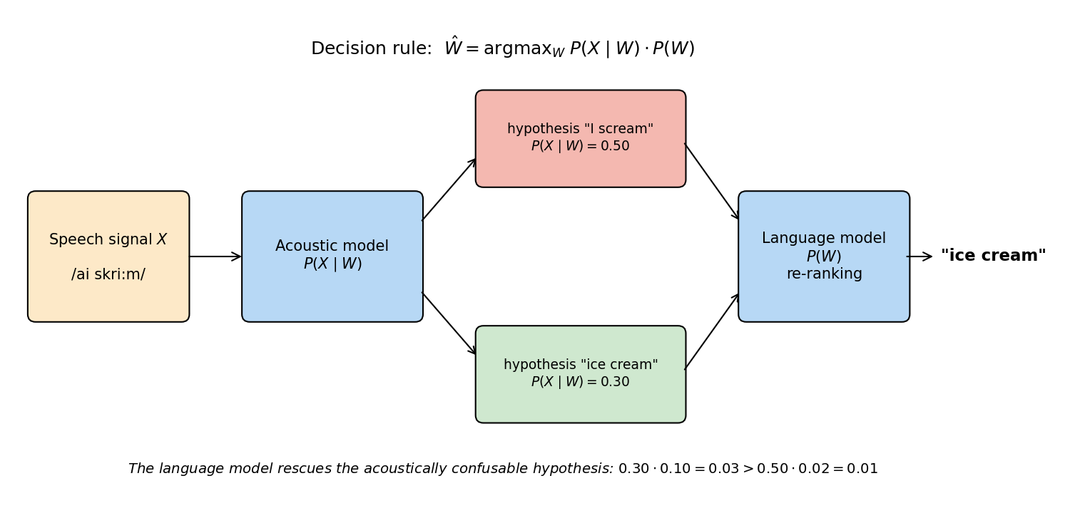
Worked comparison of two candidate sentences. The microphone recorded someone saying "recognize speech". The decoder considers two acoustically similar hypotheses:
| Hypothesis | \(P(X \mid W)\) (acoustic) | \(P(W)\) (language) | Score \(P(X \mid W) \cdot P(W)\) |
|---|---|---|---|
| \(W_1\) = "recognize speech" | \(0.30\) | \(1.00 \times 10^{-3}\) | \(3.00 \times 10^{-4}\) |
| \(W_2\) = "wreck a nice beach" | \(0.36\) | \(2.00 \times 10^{-5}\) | \(7.20 \times 10^{-6}\) |
Calculation: \(0.30 \times 0.001 = 3.00 \times 10^{-4}\) and \(0.36 \times 0.00002 = 7.20 \times 10^{-6}\).
Decision: choose \(W_1\), because \(3.00 \times 10^{-4} > 7.20 \times 10^{-6}\) — by a factor of \(3.00 \times 10^{-4} / 7.20 \times 10^{-6} \approx 41.67\). Note that \(W_2\) actually fits the audio better (higher acoustic likelihood, \(0.36 > 0.30\)), but the language model vetoes it because "wreck a nice beach" is a far less probable English utterance. This is exactly the value a language model adds.
বাংলা ব্যাখ্যা: স্পিচ রিকগনিশনে দুটো বিচারক একসাথে রায় দেয় — acoustic model বলে "শব্দতরঙ্গের সাথে কতটা মিলছে", আর language model বলে "মানুষ আদৌ এমন বাক্য বলে কি না"। উদাহরণটা দেখো: কানে "wreck a nice beach" বেশি মিললেও ভাষা মডেল জানে ওটা প্রায় কেউ বলে না, তাই "recognize speech" জেতে। দুটোর গুণফল সর্বোচ্চ যার, সেটাই চূড়ান্ত উত্তর।
1.2.5 Perplexity teaser (how language models are evaluated)
Perplexity is the standard intrinsic evaluation metric for language models (treated in depth later in the course). For a test sequence of \(N\) tokens:
Interpretation: the average branching factor — "on average, among how many equally likely words is the model hesitating at each step?" Lower is better.
Worked example on the bigram model above. We computed \(P(\text{the cat sat on the mat}) = 1/24 \approx 0.04\) with \(N = 6\) tokens:
So on this (memorized) training sentence the model is only about \(1.70\)-ways confused per word — extremely low, because the model has effectively memorized its tiny corpus. On unseen text the same model would hit a zero-probability bigram and the perplexity would be infinite. Reference points: modern Large Language Models reach single-digit perplexities on broad web text; a uniform random model over vocabulary \(V\) has perplexity exactly \(V\).
বাংলা ব্যাখ্যা: perplexity মানে — প্রতিটা ধাপে মডেল গড়ে কতগুলো শব্দের মধ্যে দ্বিধায় আছে। মান যত কম, মডেল তত আত্মবিশ্বাসী ও ভালো। আমাদের খেলনা মডেল নিজের ট্রেনিং বাক্যে ১.৭০ পায় কারণ সে কর্পাসটা মুখস্থ করে ফেলেছে; কিন্তু নতুন বাক্যে একটা শূন্য-সম্ভাবনার জোড়া পড়লেই perplexity অসীম হয়ে যায়।
From-scratch bigram language model (reference implementation)
from collections import Counter, defaultdict

corpus = "the cat sat on the mat the cat slept on the mat"
tokens = corpus.split()

unigram = Counter(tokens)
bigram = defaultdict(Counter)
for prev, curr in zip(tokens, tokens[1:]):
    bigram[prev][curr] += 1

def p_bigram(curr, prev):
    """Maximum likelihood estimate of P(curr | prev); 0.0 if unseen."""
    if unigram[prev] == 0:
        return 0.0
    return bigram[prev][curr] / unigram[prev]

print("P(cat | the) =", p_bigram("cat", "the"))   # 2 / 4 = 0.5
print("P(mat | the) =", p_bigram("mat", "the"))   # 2 / 4 = 0.5
print("P(sat | cat) =", p_bigram("sat", "cat"))   # 1 / 2 = 0.5

def score(sentence):
    """Product of bigram probabilities (first-word prior omitted here)."""
    toks = sentence.split()
    p = 1.0
    for prev, curr in zip(toks, toks[1:]):
        p *= p_bigram(curr, prev)
    return p

print("score('the cat sat')    =", score("the cat sat"))     # 0.5 * 0.5 = 0.25
print("score('the mat sat on') =", score("the mat sat on"))  # contains unseen pair -> 0.0
Algorithm summary: tokenize → count unigrams and bigrams in one pass (\(O(N)\) time) → divide counts. Worst-case memory \(O(V^2)\) for the bigram table. Strengths: trivial, interpretable. Weaknesses: zero counts, no generalization, vocabulary explosion.
Section 1.3 — Large Language Models
What the slides say
- A Large Language Model is a massive neural language model: the same next-word objective as Section 1.2, but parameterized by a deep neural network.
- Training data: trillions of tokens from the open web (Common Crawl, books, source code).
- Scale: billions to hundreds of billions of parameters; pretraining costs tens of millions of dollars in compute.
- Large Language Models are general purpose: one model can summarize, translate, write code, and chat.
Technical explanation
- Architecture: decoder-only Transformer (details in Chapter 2).
- Training objective: maximize \(\sum_t \log P_\theta(w_t \mid w_{<t})\) over a giant corpus — exactly the chain rule from 1.2.1, with the conditional implemented by a neural network with parameters \(\theta\) instead of count tables.
- Inference: autoregressive generation — sample or select one token, append it to the context, repeat.
- Capabilities emerge with scale: a small language model cannot write a coherent poem; a 70-billion-parameter model can, without any poem-specific training.
Why a neural network instead of counts
A neural language model represents words as continuous vectors, so "cat" and "dog" share statistical strength; attention lets it use context windows of thousands of tokens instead of \(n - 1\); and its memory is fixed at the parameter count instead of exploding as \(V^n\). It solves precisely the three failures of n-grams from 1.2.3.
Autoregressive generation in ten lines
import random
random.seed(0)

# Mock conditional distribution: prefix -> weighted next-word candidates
mock_lm = {
    "I":         [("love", 0.6), ("am", 0.3), ("hate", 0.1)],
    "I love":    [("AI", 0.5), ("you", 0.4), ("Python", 0.1)],
    "I love AI": [(".", 0.7), ("!", 0.3)],
}

def sample_next(prefix):
    if prefix not in mock_lm:
        return "."
    words, probs = zip(*mock_lm[prefix])
    return random.choices(words, weights=probs, k=1)[0]

def generate(prefix, max_steps=5):
    for _ in range(max_steps):
        nxt = sample_next(prefix)
        prefix = (prefix + " " + nxt).strip()
        if nxt in {".", "!"}:
            break
    return prefix

print(generate("I"))   # e.g. "I love AI ."
Replace the dictionary with a Transformer's next-token distribution and this is GPT-style decoding.
Common mistakes
- Thinking Large Language Models "look up" facts — they store statistics in their weights; they do not query a database (that gap is what Retrieval-Augmented Generation in Chapter 4 fixes).
- Believing they cannot be wrong — hallucination (fluent but false output) is an inherent failure mode.
Exam relevance
- Definition question: Large Language Model = neural language model + Transformer architecture + web-scale pretraining data + autoregressive generation + general-purpose capabilities.
- Contrast question: count-based n-gram vs. neural language model (memory, generalization, context length, interpretability).
বাংলা ব্যাখ্যা: Large Language Model আসলে সেই পুরনো "পরের শব্দ অনুমান" মডেলই — পার্থক্য হলো গণনার টেবিলের জায়গায় বিশাল নিউরাল নেটওয়ার্ক, আর খেলনা কর্পাসের জায়গায় প্রায় গোটা ইন্টারনেট। শব্দগুলো ভেক্টর হিসেবে থাকে বলে "cat" আর "dog"-এর মিল মডেল নিজেই বোঝে — n-gram-এর তিনটা বড় দুর্বলতাই এতে দূর হয়। তবে মনে রেখো: মডেল তথ্য "খুঁজে দেখে না", ওজনের ভেতরে জমা পরিসংখ্যান থেকে বলে — তাই hallucination হয়।
Section 1.4 — Foundation Models
What the slides say
- A Foundation Model is a single, large model pretrained on broad data with self-supervision that can be adapted to a wide range of downstream tasks.
- The term was coined by the Stanford Center for Research on Foundation Models in 2021.
- Foundation models exist across modalities: text (Large Language Models), images (diffusion models such as Stable Diffusion and DALL-E), audio (Whisper), video (Sora), and multimodal combinations (GPT-4o, Gemini).
- The defining property is the pretrain → adapt workflow: one expensive pretraining run, then many cheap adaptations.
The paradigm shift
Classical machine learning: one task → collect labelled data for that task → train a task-specific model → deploy. Every new task restarts the pipeline.
Foundation-model era: pretrain once on broad unlabelled data → adapt cheaply per task via prompting (Chapter 3), retrieval (Chapter 4), tool use and agents (Chapter 5), or fine-tuning (Chapter 6).
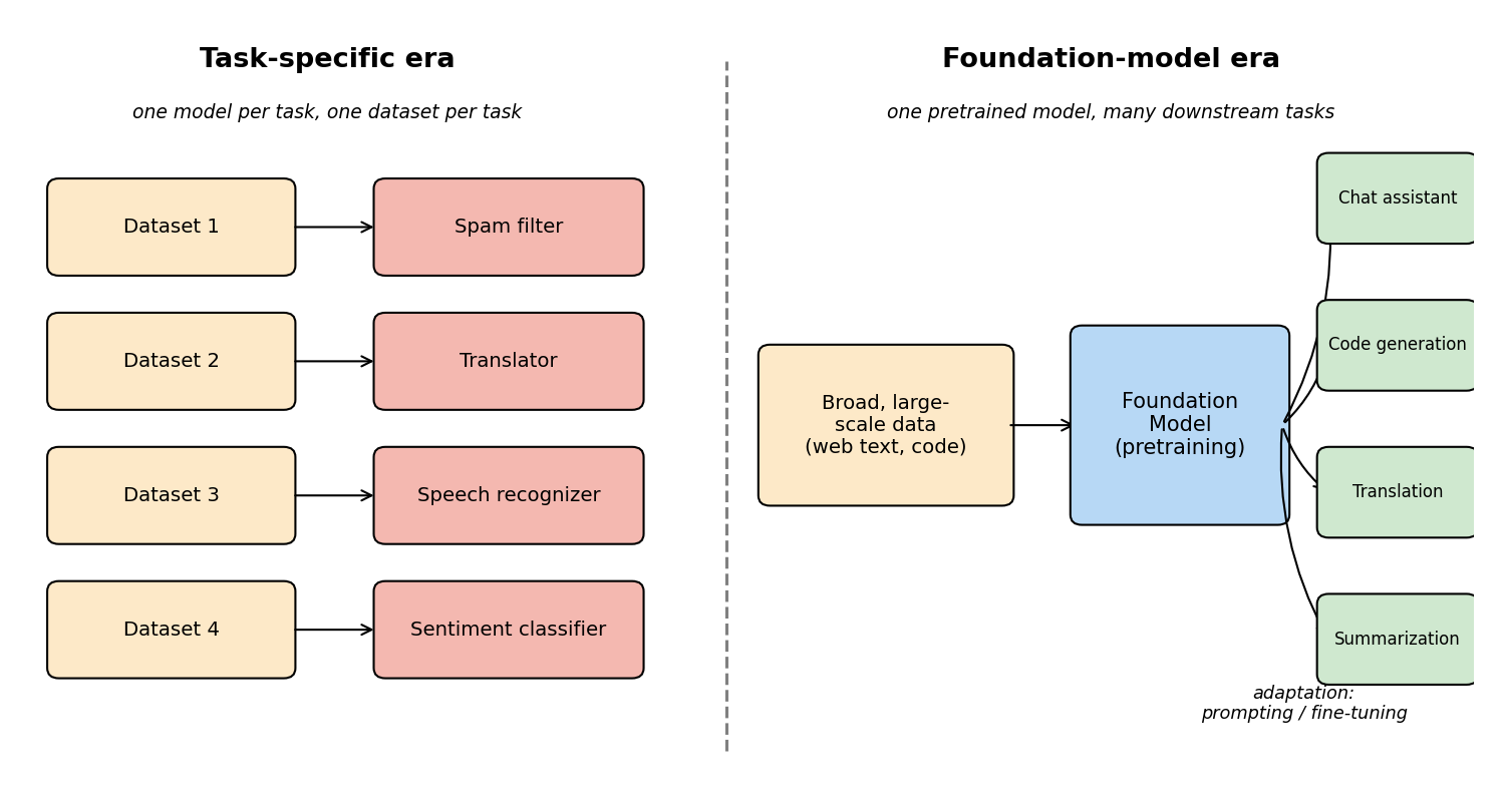
The economic consequence defines this course: because pretraining costs tens of millions of dollars, almost nobody trains foundation models — almost everybody engineers products on top of them. That activity is AI Engineering.
Adaptation by prompting in one picture
# One "model", two different tasks, selected purely by the system prompt.
def fake_llm(system, user):
    return f"[mode={system!r}] processed: {user.upper()}"

print(fake_llm(system="You are a translator. Translate to French.",
               user="Hello world"))
print(fake_llm(system="You are a sentiment classifier. Reply POSITIVE or NEGATIVE.",
               user="I love this lecture"))
The same function plays two roles; the task selection happens entirely through the prompt. This adaptation without retraining is the defining capability of foundation models.
Common mistakes
- Treating "Foundation Model" as a synonym for "Large Language Model" — Large Language Models are one type of foundation model (the text modality).
- Assuming adaptation always means retraining — often a prompt is enough.
Exam relevance
- Definition question (use the three keywords: broad data, self-supervision, adaptable to many downstream tasks).
- Mini-case: "A startup needs a legal-document summarizer and a support chatbot. Classical approach vs. foundation-model approach?" — technique: one pretrained foundation model adapted twice (prompting or fine-tuning); justification: shared pretraining cost, faster time to market, transfer of general language competence; trade-off: dependence on the model provider, less control over failure modes, inference cost.
বাংলা ব্যাখ্যা: আগের যুগে প্রতিটা কাজের জন্য আলাদা ডেটা জোগাড় করে আলাদা মডেল বানাতে হতো; এখন একটা বিশাল মডেল একবার পূর্বপ্রশিক্ষণ (pretraining) করে নানা কাজে অভিযোজন করা হয়। অভিযোজনের চারটা রাস্তা — prompt লেখা, বাইরের তথ্য জোড়া (retrieval), টুল ব্যবহার (agent), আর fine-tuning — এগুলোই এই কোর্সের অধ্যায় ৩ থেকে ৬। যেহেতু pretraining-এর খরচ কোটি ডলার, তাই বাস্তবের কাজ হলো তৈরি মডেলের ওপর প্রোডাক্ট বানানো — এটাই AI Engineering।
Section 1.5 — Examples Across Modalities and Tools
What the slides say
- Image generation: DALL-E, Stable Diffusion — text prompt in, image out (diffusion models, a non-autoregressive family of foundation models).
- Video generation: Sora, Runway.
- Code generation: GitHub Copilot, Cursor — Large Language Models trained heavily on source code; "vibe coding" as the buzzword for prompt-driven development.
- Local inference: Ollama lets you run open-weight models (for example LLaMA-3 8B) on a laptop; quantization (4-bit / 8-bit integer weights) makes the model fit in consumer memory.
- Frameworks: LangChain and LangFlow glue models, prompts, retrieval, and tools together behind a Python application programming interface.
Minimal local-inference example (as shown in the lecture)
# pip install ollama          (and:  ollama pull llama3.1:8b  — about 4 GB)
# Illustrative; requires a running Ollama installation.
# import ollama
# resp = ollama.chat(
#     model="llama3.1:8b",
#     messages=[{"role": "user", "content": "What is a foundation model?"}],
# )
# print(resp["message"]["content"])

# Offline-safe stand-in with the same interface:
def call_local_llm(model, prompt):
    return f"[{model}] would answer: {prompt}"

print(call_local_llm("llama3.1:8b", "What is a foundation model?"))
Three lines of real code give you a private, offline assistant — that is the premise of local inference.
Common mistakes
- Assuming "running locally" is free — it costs memory, graphics-processing-unit time, and electricity, and a quantized 8-billion-parameter model is far weaker than a frontier model.
- Confusing LangChain (a software framework) with the model — LangChain contains no intelligence; it orchestrates calls to models.
Exam relevance
- Short answer: "What is Ollama?" — a runtime for local execution of open-weight Large Language Models.
- "Name two foundation models of different modalities" — for example Stable Diffusion (image) and Whisper (audio).
- Trade-off question: local inference (privacy up, capability and convenience down) versus hosted application programming interfaces (capability up, data leaves the premises, per-token cost).
বাংলা ব্যাখ্যা: এই সেকশনটা মূলত প্রোডাক্ট-ভ্রমণ: ছবি বানায় diffusion মডেল, কোড লেখে কোড-কর্পাসে শেখা ভাষা মডেল, আর Ollama দিয়ে নিজের ল্যাপটপেই ছোট মডেল চালানো যায়। পরীক্ষার জন্য মূল trade-off-টা মনে রাখো — লোকালে চালালে গোপনীয়তা বাড়ে কিন্তু সক্ষমতা কমে; ক্লাউড মডেলে উল্টোটা।
Section 1.6 — Lecture Overview and Organization
Course map
| # | Chapter | Goal |
|---|---|---|
| 1 | Introduction | Motivation, vocabulary, the foundation-model paradigm |
| 2 | Foundation Models | How Large Language Models work internally |
| 3 | Prompt Engineering | Controlling model outputs through inputs |
| 4 | Retrieval-Augmented Generation | Connecting models to external knowledge |
| 5 | Agents | Autonomous, tool-using systems |
| 6 | Fine-tuning | Adapting model weights to specific tasks |
| 7 | Legal and Ethical Aspects | Responsibilities, risks, regulation |
| 8 | Building Applications | Putting it all together in practice |
Organization
- Laboratory schedule: 5 units accompanying the lecture.
- Prerequisites: Pattern Recognition and the AI Engineering laboratory.
- Recommended literature: Chip Huyen, “AI Engineering”, O'Reilly, ISBN 978-1-098-16630-4.
Exam relevance
- Matching question: chapter number ↔ topic (cheap points — memorize the table).
- The chapter map also explains why the course is ordered this way: understand the model (2), then steer it (3), ground it (4), let it act (5), specialize it (6), and deploy it responsibly (7–8).
বাংলা ব্যাখ্যা: কোর্সের গল্পটা একটা সিঁড়ির মতো — আগে মডেলটা ভেতর থেকে বোঝো (অধ্যায় ২), তারপর prompt দিয়ে চালাও (৩), বাইরের জ্ঞান জুড়ে দাও (৪), কাজ করতে দাও (৫), দরকারে ওজন বদলাও (৬), শেষে আইন-নৈতিকতা মেনে প্রোডাক্ট নামাও (৭–৮)। টেবিলটা মুখস্থ রাখলে ম্যাচিং প্রশ্নে সহজ নম্বর।
5. Algorithm Box — Bigram Maximum Likelihood Language Model
Problem: estimate \(\hat P(w_t \mid w_{t-1})\) from a training corpus, then score new sentences. This is the only complete algorithm of Chapter 1 and a very likely template for the numerical exam question.
Pseudocode:
function TRAIN(corpus):
    tokens  <- split(corpus)                     # whitespace tokenization
    unigram <- empty counter
    bigram  <- empty nested counter
    for each token w in tokens:
        unigram[w] <- unigram[w] + 1
    for each adjacent pair (prev, curr) in tokens:
        bigram[prev][curr] <- bigram[prev][curr] + 1
    return unigram, bigram, length(tokens)

function PROB(prev, curr):
    if unigram[prev] = 0:  return 0
    return bigram[prev][curr] / unigram[prev]    # maximum likelihood estimate

function SCORE(sentence):                        # base-2 log probability
    toks <- split(sentence)
    logp <- log2( unigram[first(toks)] / n_tokens )
    for each adjacent pair (prev, curr) in toks:
        p <- PROB(prev, curr)
        if p = 0:  return -infinity              # zero-count problem
        logp <- logp + log2(p)
    return logp
Dry run of SCORE("the cat sat") on the toy corpus from 1.2.2 (12 tokens):
| Step | Term | Count ratio | Probability | Running product |
|---|---|---|---|---|
| start | \(P(\text{the})\) | \(4/12\) | \(0.33\) | \(0.33\) |
| 1 | \(\hat P(\text{cat} \mid \text{the})\) | \(2/4\) | \(0.50\) | \(0.17\) |
| 2 | \(\hat P(\text{sat} \mid \text{cat})\) | \(1/2\) | \(0.50\) | \(0.08\) |
Result: \(P(\text{the cat sat}) = 1/12 \approx 0.08\), i.e. \(\log_2 P = -3.58\).
Complexity: training is a single pass, \(O(N)\) time in the corpus length \(N\); the bigram table needs at most \(O(V^2)\) memory for vocabulary size \(V\) (in practice far less, because most pairs never occur).
Strengths: trivial to implement, fully interpretable, exact counts. Weaknesses: zero probability for unseen pairs, no generalization across similar words, table explosion for higher-order n-grams.
Typical implementation bugs (also exam traps): dividing by the corpus length or vocabulary size instead of \(C(w_{t-1})\); forgetting the start term; multiplying raw probabilities until floating-point underflow instead of summing logarithms; silently treating an unseen pair as "skip" instead of probability zero.
বাংলা ব্যাখ্যা: অ্যালগরিদমটা তিন ধাপের: একবার কর্পাস পড়ে গোনো, ভাগ করে সম্ভাবনা বানাও, তারপর নতুন বাক্যে লগারিদম যোগ করে স্কোর দাও। dry run টেবিলটা হাতে-কলমে অনুশীলন করো — পরীক্ষায় ঠিক এই ছকেই হিসাব দেখালে আংশিক নম্বরও নিশ্চিত থাকে, কোথাও ভুল হলেও ধাপগুলো স্পষ্ট দেখা যায়।
6. Mapped Notebooks — What to Take From Them
| Notebook | Role for Chapter 1 | Minimum skill to extract |
|---|---|---|
0-1-python-basics.ipynb |
Prerequisite refresher: variables, loops, functions, comprehensions, classes | Read and write a for loop over zip(tokens, tokens[1:]) without hesitation |
0-2-files-and-data.ipynb |
Loading text, JSON, and CSV data; streaming large files line by line | Load a text corpus from disk before counting n-grams |
0-3-pytorch-intro.ipynb |
Tensors, automatic differentiation, modules, training loops | Needed from Chapter 2 onwards (neural language models) |
0-4-pytorch-advanced.ipynb |
Custom layers, data loaders, checkpointing, mixed precision | Needed for Chapter 6 (fine-tuning) |
Self-test linked to this chapter — write the following function from memory:
from collections import Counter

def bigram_prob(corpus: str, prev: str, curr: str) -> float:
    """Return the maximum likelihood estimate of P(curr | prev)."""
    toks = corpus.split()
    pair_counts = Counter(zip(toks, toks[1:]))
    word_counts = Counter(toks)
    return pair_counts[(prev, curr)] / word_counts[prev] if word_counts[prev] else 0.0
If you can write this in under three minutes, the coding part of the Chapter 1 exam material holds no danger for you.
বাংলা ব্যাখ্যা: নোটবুকগুলোর মধ্যে এই অধ্যায়ের জন্য আসল কাজের জিনিস হলো Python-এর সাবলীলতা — বিশেষ করে zip(tokens, tokens[1:]) দিয়ে পাশাপাশি জোড়া বানানোর কৌশলটা। ওপরের ফাংশনটা না দেখে লিখতে পারা মানে Chapter 1-এর কোডিং অংশ তোমার আয়ত্তে।
7. Real-Life Applications
| Application | How Chapter 1 ideas are used | Limitation |
|---|---|---|
| Mobile keyboard autocomplete | Bigram / n-gram or a small neural language model | Limited context, weak on rare phrases |
| Speech recognition (Siri, Alexa, Whisper) | Language-model rescoring of acoustic hypotheses (noisy channel) | Language-model bias can "correct" rare names away |
| Search-engine query suggestions | Language model over query logs | Privacy-sensitive data |
| Customer-support bot | Foundation model + retrieval (Chapter 4) + tools (Chapter 5) | Hallucination risk |
| Code assistant (Copilot, Cursor) | Large Language Model trained on source code | Licensing and intellectual-property questions |
| Medical scribing | Large Language Model summarizing dictation | Legal liability (Chapter 7) |
বাংলা ব্যাখ্যা: খেয়াল করো — টেবিলের প্রতিটা প্রোডাক্টের গভীরে সেই একই গণিত: শব্দের ধারার সম্ভাবনা। কীবোর্ড সাজেশন থেকে শুরু করে মেডিকেল নোট লেখা পর্যন্ত সবই language modelling-এর প্রয়োগ, শুধু মডেলের আকার আর চারপাশের প্রকৌশল আলাদা।
8. Exam-Focused Summary
| Topic | What to be able to reproduce |
|---|---|
| ChatGPT acronym | Chat (interface), Generative, Pretrained, Transformer (architecture) |
| Chain rule | \(P(w_1,\ldots,w_T) = \prod_{t=1}^{T} P(w_t \mid w_1,\ldots,w_{t-1})\) — exact, no approximation |
| Bigram estimate | \(\hat P(w_t \mid w_{t-1}) = C(w_{t-1}, w_t)\,/\,C(w_{t-1})\) — denominator = count of the previous word |
| Speech-recognition decision rule | \(\hat W = \arg\max_W P(X \mid W)\,P(W)\); acoustic model × language model; \(P(X)\) dropped because it is constant |
| Perplexity | \(\mathrm{PPL} = P(w_{1..N})^{-1/N}\); average branching factor; lower is better |
| Foundation Model | Pretrained on broad data with self-supervision, adaptable to many downstream tasks |
| Course outline | 8 chapters — be able to list them |
What to memorize: the glossary, the four formulas, the course outline. What to understand deeply: the chain rule, the zero-count problem, why scale plus transfer produces the foundation-model paradigm. What to practice on paper: bigram counting with a fresh toy corpus, the speech-recognition product comparison, one perplexity computation.
Common traps:
- Wrong denominator in the bigram maximum likelihood estimate.
- Mixing up which letter of "Generative Pretrained Transformer" is the architecture.
- Treating chat memory as a model property (it is an application-layer construct).
- Equating Large Language Model with Foundation Model (subset, not synonym).
- Forgetting that one zero-probability bigram makes the whole sentence probability zero.
বাংলা ব্যাখ্যা: পরীক্ষার আগের রাতে এই টেবিলটাই যথেষ্ট — চারটা সূত্র (chain rule, bigram estimate, Bayes decision rule, perplexity), শব্দভান্ডার, আর আটটা অধ্যায়ের তালিকা। হিসাবের প্রশ্নে সবচেয়ে বেশি নম্বর কাটা যায় ভুল ভাজকে আর শূন্য-সম্ভাবনা খেয়াল না করায় — এই দুটো জায়গায় দুবার করে চেক দিও।
9. Deep-Thinking Questions (with short model answers)
These go slightly beyond the slides — the level a TU Braunschweig examiner reaches for when separating a 1.0 from a 2.0.
Q1. Why did next-word prediction — a seemingly trivial objective — produce models capable of translation, mathematics, and reasoning? Answer: to predict the next word better than chance on web-scale text, a model must internally represent grammar (subject-verb agreement), world facts ("Paris is in France"), arithmetic patterns, and discourse structure ("…therefore the answer is…"). Next-word prediction is therefore an implicit multi-task objective; at sufficient scale, the optimal predictor is a generalist. "It just memorizes" is the wrong answer — held-out benchmarks contain items that never appear in the training data.
Q2. Derive the chain rule of language modelling from the definition of conditional probability. Answer: by definition, \(P(A, B) = P(A)\,P(B \mid A)\). Apply it recursively to the joint distribution:
No independence assumption is used anywhere — the chain rule is exact; approximations only enter when the history is truncated (Markov assumption).
Q3. A friend claims "ChatGPT is conscious because it remembers our conversation." Refute this using Section 1.1. Answer: the model is stateless; the chat application re-sends the entire conversation history as context with every request. Apparent memory is an application-layer construct, bounded by the context length — it provides no evidence about consciousness.
Q4. Compare a 5-gram model and a Transformer-based Large Language Model along memory, generalization, and interpretability. Answer: memory — the 5-gram table grows toward \(O(V^5)\) while the Transformer has a fixed parameter budget; generalization — the 5-gram treats "the cat sat" and "the dog sat" as unrelated events, while continuous word representations share statistical strength; interpretability — the 5-gram is fully transparent (counts), the Transformer is largely a black box. The trade-off is transparency versus capability.
Q5. What happens to a speech recognizer if the language model is removed (set \(P(W)\) uniform)? Answer: the decision rule degenerates to \(\arg\max_W P(X \mid W)\) — pure acoustic matching. Homophone confusions explode: "wreck a nice beach" beats "recognize speech" whenever it fits the audio marginally better (see the worked table in 1.2.4, where the acoustic model alone would have chosen the wrong hypothesis).
Q6. Why can a bigram model trained on a 1-gigabyte out-of-domain corpus perform worse than one trained on 10 megabytes of in-domain text? Answer: probability mass follows the training domain. The large out-of-domain model assigns zero (or near-zero, after smoothing) probability to the test domain's characteristic word pairs, while the small in-domain model covers exactly those pairs. Data relevance beats data volume — the same argument later motivates domain-specific fine-tuning (Chapter 6) and retrieval (Chapter 4).
Q7. Both a diffusion image model and a decoder-only Transformer count as foundation models. What do they share, given that their architectures differ completely? Answer: the paradigm, not the architecture: broad-data pretraining with self-supervision, followed by cheap adaptation to many downstream tasks. The definition of a foundation model is a statement about the training-and-use workflow, not about any particular network design.
বাংলা ব্যাখ্যা: এই প্রশ্নগুলোর ধরন খেয়াল করো — প্রতিটাই "কেন" বা "তুলনা করো" জাতীয়, আর প্রতিটার উত্তর লেকচারের কোনো না কোনো মূল ধারণায় (statelessness, chain rule, zero-count, pretrain→adapt) ফিরে যায়। মৌখিক বা লিখিত — যেকোনো পরীক্ষায় কঠিন প্রশ্ন মানে নতুন তথ্য নয়, পুরনো ধারণার নতুন প্রয়োগ।
Mock Exam — Chapter 1
Instructions: 50 points total, modeled on the real format (120 minutes for a full exam; budget about 55–60 minutes for this chapter set). Answer in English. Use the technical terms from the lecture. Do not use abbreviations. Round all numerical results to 2 decimal places. A non-programmable calculator is allowed.
Level 1 — Basic (8 points)
Q1.1 (1 pt). Which statement best describes a Foundation Model?
- (a) Any neural network with more than one billion parameters.
- (b) A model pretrained on broad data with self-supervision that can be adapted to a wide range of downstream tasks.
- (c) A rule-based expert system that forms the base layer of a software stack.
- (d) A language model that has been fine-tuned exclusively for conversational chat.
Q1.2 (1 pt). Which statement best describes the role of the language model \(P(W)\) in the speech-recognition decision rule \(\hat W = \arg\max_W P(X \mid W)\,P(W)\)?
- (a) It converts the raw audio signal into acoustic feature vectors.
- (b) It models how well the audio evidence matches a given word sequence.
- (c) It assigns a prior probability to each candidate word sequence, favoring linguistically plausible hypotheses.
- (d) It normalizes the posterior by dividing by the evidence \(P(X)\).
Q1.3 (1 pt). Which statement best describes the meaning of "Transformer" within "Generative Pretrained Transformer"?
- (a) It names the conversational user interface of the product.
- (b) It names the large-scale first training stage on web data.
- (c) It names the attention-based neural network architecture of the model.
- (d) It names the decoding strategy used to sample output tokens.
Q1.4 (1 pt). Which statement best describes the first-order Markov assumption made by a bigram language model?
- (a) Every word in the sentence is statistically independent of every other word.
- (b) The probability of the next word depends only on the immediately preceding word.
- (c) The probability of the next word depends on the entire preceding history.
- (d) The probability of a word depends on the word that follows it.
Q1.5 (2 pts). Define the term token and give one example of a word that is split into more than one token.
Q1.6 (2 pts). Define autoregressive generation and state the two repeated steps of the generation loop.
Level 2 — Intuitive Analysis (6 points)
Q2.1 (3 pts). Explain why a maximum-likelihood bigram language model assigns probability zero to many grammatically correct sentences. Structure your answer as cause → mechanism → consequence.
Q2.2 (3 pts). Explain why training a model only on next-word prediction can nevertheless produce a system that translates, summarizes, and answers questions without task-specific training. Structure your answer as cause → mechanism → consequence.
Level 3 — Numerical Application (10 points)
Q3.1 (5 pts). Given the training corpus (treat it as one continuous token stream, no sentence boundaries):
students love deep learning students love language models students study deep learning
(a) Compute the maximum likelihood estimates \(\hat P(\text{love} \mid \text{students})\), \(\hat P(\text{deep} \mid \text{love})\), and \(\hat P(\text{learning} \mid \text{deep})\). (b) Using the unigram probability of the first word as the start term, compute the bigram-model probability of the sentence "students love deep learning". (c) Compute the perplexity of this sentence under the model (\(N = 4\) tokens).
Q3.2 (5 pts). A speech recognizer must decide between two hypotheses for one utterance \(X\):
| Hypothesis | \(P(X \mid W)\) | \(P(W)\) |
|---|---|---|
| \(W_1\) = "I scream" | \(0.42\) | \(3.00 \times 10^{-4}\) |
| \(W_2\) = "ice cream" | \(0.35\) | \(1.00 \times 10^{-3}\) |
(a) Write down the Bayes decision rule used in automatic speech recognition and explain why \(P(X)\) may be omitted. (b) Compute the decision score for both hypotheses and state which sentence the recognizer outputs. (c) One hypothesis fits the audio better but still loses. Name the component responsible and explain its effect in one sentence.
Level 4 — Transfer (8 points)
Q4.1 (4 pts). Zero-count problem and smoothing. Using the corpus from Q3.1 (vocabulary size \(V = 7\)): (a) Show that the maximum likelihood estimate \(\hat P(\text{models} \mid \text{love})\) is zero. (b) Compute the Laplace (add-one) smoothed estimates \(\hat P_{\mathrm{Laplace}}(\text{models} \mid \text{love})\) and \(\hat P_{\mathrm{Laplace}}(\text{deep} \mid \text{love})\) using \(\hat P_{\mathrm{Laplace}}(w \mid w') = \frac{C(w', w) + 1}{C(w') + V}\). (c) State one benefit and one drawback of Laplace smoothing.
Q4.2 (4 pts). Classical statistics often assumes data points are independent and identically distributed. Explain why this assumption fails for natural-language text, and state the modelling consequence drawn in this lecture. Give one concrete example where word order changes the meaning.
Level 5 — Coding (18 points)
Q5.1 (9 pts). Write a Python program that (a) trains a bigram language model with maximum likelihood estimation on the corpus "the cat sat on the mat the cat slept on the mat", (b) prints \(P(\text{cat} \mid \text{the})\), \(P(\text{mat} \mid \text{the})\), and \(P(\text{sat} \mid \text{cat})\), (c) computes the base-2 log probability of a sentence (using the unigram probability of the first word as the start term), and (d) computes the perplexity. Demonstrate it on "the cat sat on the mat" and on "the mat sat on the cat", and explain the second result.
Q5.2 (9 pts). Extend Q5.1 with Laplace (add-one) smoothing of the bigram probabilities (keep the unsmoothed unigram start term). Print the vocabulary size, the smoothed probabilities \(P_{\mathrm{Laplace}}(\text{sat} \mid \text{mat})\) and \(P_{\mathrm{Laplace}}(\text{cat} \mid \text{the})\), and the base-2 log probability and perplexity of both test sentences from Q5.1. Explain what changed and why.
Solutions
Level 1 Solutions
Q1.1 — (b). A Foundation Model is defined by broad pretraining data, self-supervised training, and adaptability to many downstream tasks. (a) is wrong because parameter count alone does not define the paradigm; (c) describes classical symbolic systems; (d) describes one adapted product, not the foundation itself.
Q1.2 — (c). The language model is the prior over word sequences: it scores linguistic plausibility independently of the audio. (a) is feature extraction, (b) is the acoustic model \(P(X \mid W)\), (d) is unnecessary because \(P(X)\) is constant across hypotheses and cancels in the \(\arg\max\).
Q1.3 — (c). Transformer names the attention-based architecture ("Attention is All You Need", 2017). Chat is the interface (a), Pretrained is the training stage (b), and the decoding strategy (d) is not part of the acronym at all.
Q1.4 — (b). The bigram model truncates the chain-rule history to the single preceding token: \(P(w_t \mid w_1,\ldots,w_{t-1}) \approx P(w_t \mid w_{t-1})\). (a) is the unigram/independence assumption, (c) is the exact chain rule without approximation, (d) reverses the direction of conditioning.
Q1.5 — Token. A token is the smallest input unit a language model processes — a word, sub-word fragment, or byte sequence, drawn from a fixed vocabulary. Example: "playing" → ["play", "ing"]. (1 pt definition, 1 pt example.)
Q1.6 — Autoregressive generation. Generating a sequence one token at a time, where each new token is conditioned on all previously generated tokens. The loop: (1) compute the probability distribution over the vocabulary given the current context, select or sample one token; (2) append that token to the context and repeat until a stop condition. (1 pt definition, 1 pt loop.)
Level 2 Solutions
Q2.1. - Cause: Every training corpus is finite, so many valid word pairs of the language never occur in it. - Mechanism: The maximum likelihood estimate is a count ratio, \(\hat P(w \mid w') = C(w', w)/C(w')\); an unseen pair has \(C(w', w) = 0\), hence probability \(0.00\), and because the sentence probability is a product of bigram probabilities, a single zero factor forces the entire sentence probability to \(0.00\). - Consequence: The model cannot rank or accept unseen-but-grammatical sentences (perplexity becomes infinite), which is fatal in applications such as speech-recognition rescoring; this motivates smoothing techniques and, ultimately, neural language models that generalize across similar words.
Q2.2. - Cause: Web-scale training corpora implicitly contain demonstrations of countless tasks — parallel translations, summaries next to articles, questions followed by answers. - Mechanism: To keep reducing next-word prediction loss on such data, the model is forced to internalize grammar, world facts, and cross-language and cross-format regularities; next-word prediction therefore acts as an implicit multi-task objective. - Consequence: At sufficient scale, the capabilities transfer: the model performs translation or summarization zero-shot, without task-specific training — this transfer property is exactly what makes the foundation-model paradigm work.
Level 3 Solutions
Q3.1. The corpus has 12 tokens. Relevant counts: \(C(\text{students}) = 3\), \(C(\text{love}) = 2\), \(C(\text{deep}) = 2\); bigram counts \(C(\text{students love}) = 2\), \(C(\text{love deep}) = 1\), \(C(\text{deep learning}) = 2\).
(a) Maximum likelihood estimates (2 pts):
(b) Start term: \(P(\text{students}) = 3/12 = 0.25\). Sentence probability (2 pts):
(c) Perplexity with \(N = 4\) (1 pt):
(Check via logs: \(\log_2(1/12) = -3.58\); \(\mathrm{PPL} = 2^{3.58/4} = 2^{0.90} \approx 1.86\).)
Q3.2. (a) Decision rule (1 pt): \(\hat W = \arg\max_W P(W \mid X) = \arg\max_W P(X \mid W)\,P(W)\). The evidence \(P(X)\) is identical for every hypothesis (the audio is fixed), so dividing by it does not change which hypothesis attains the maximum — it may be omitted from the \(\arg\max\) (1 pt).
(b) Scores (2 pts):
Since \(3.50 \times 10^{-4} > 1.26 \times 10^{-4}\), the recognizer outputs \(W_2\) = "ice cream".
(c) (1 pt) \(W_1\) fits the audio better (\(0.42 > 0.35\)) but loses because of the language model \(P(W)\): it rates "ice cream" as a far more probable utterance than "I scream", and this prior outweighs the small acoustic advantage.
Level 4 Solutions
Q4.1. (a) The bigram "love models" never occurs in the corpus: \(C(\text{love models}) = 0\), so \(\hat P(\text{models} \mid \text{love}) = 0/2 = 0.00\) (1 pt).
(b) With \(C(\text{love}) = 2\) and \(V = 7\) (2 pts):
(c) (1 pt) Benefit: no event has probability zero, so unseen-but-valid sentences keep a nonzero probability and perplexity stays finite. Drawback: probability mass is taken away from observed events and spread uniformly over all \(V\) continuations; with a large vocabulary and a small corpus this over-smooths — note how the seen bigram dropped from \(0.50\) to \(0.22\).
Q4.2. - Cause: Natural language is produced sequentially with strong structural constraints — syntax, agreement, topical coherence — so neighboring words are heavily dependent on one another. - Mechanism: Independence fails because \(P(w_t)\) changes drastically with the history (\(P(\text{learning} \mid \text{deep}) = 1.00\) versus the unconditional \(P(\text{learning}) = 0.17\) in the Q3.1 corpus); identical distribution fails because the distribution over words shifts with position, topic, and domain. - Consequence (lecture's conclusion): Text must be modelled with the chain rule using conditional models, \(P(w_1,\ldots,w_T) = \prod_t P(w_t \mid w_{<t})\) — this is exactly what language models are. Word-order example: "the dog bites the man" versus "the man bites the dog" — identical bag of words, opposite meaning, so any order-blind independence model assigns them the same probability.
Level 5 Solutions
Q5.1 — Complete solution code (verified by execution):
import math
from collections import Counter, defaultdict

def train_bigram(corpus):
    tokens = corpus.split()
    unigram = Counter(tokens)
    bigram = defaultdict(Counter)
    for prev, curr in zip(tokens, tokens[1:]):
        bigram[prev][curr] += 1
    return unigram, bigram, len(tokens)

def bigram_prob(prev, curr, unigram, bigram):
    if unigram[prev] == 0:
        return 0.0
    return bigram[prev][curr] / unigram[prev]

def sentence_logprob(sentence, unigram, bigram, n_tokens):
    toks = sentence.split()
    logp = math.log2(unigram[toks[0]] / n_tokens)   # unigram start term
    for prev, curr in zip(toks, toks[1:]):
        p = bigram_prob(prev, curr, unigram, bigram)
        if p == 0.0:
            return float("-inf")                    # one zero kills the product
        logp += math.log2(p)
    return logp

def perplexity(sentence, unigram, bigram, n_tokens):
    logp = sentence_logprob(sentence, unigram, bigram, n_tokens)
    n = len(sentence.split())
    if logp == float("-inf"):
        return float("inf")
    return 2.0 ** (-logp / n)

corpus = "the cat sat on the mat the cat slept on the mat"
unigram, bigram, n_tokens = train_bigram(corpus)

print(f"P(cat | the) = {bigram_prob('the', 'cat', unigram, bigram):.2f}")
print(f"P(mat | the) = {bigram_prob('the', 'mat', unigram, bigram):.2f}")
print(f"P(sat | cat) = {bigram_prob('cat', 'sat', unigram, bigram):.2f}")

s1 = "the cat sat on the mat"
s2 = "the mat sat on the cat"
lp1 = sentence_logprob(s1, unigram, bigram, n_tokens)
print(f"log2 P(s1) = {lp1:.2f}")
print(f"P(s1)      = {2.0**lp1:.4f}")
print(f"PPL(s1)    = {perplexity(s1, unigram, bigram, n_tokens):.2f}")
print(f"log2 P(s2) = {sentence_logprob(s2, unigram, bigram, n_tokens)}")
print(f"PPL(s2)    = {perplexity(s2, unigram, bigram, n_tokens)}")
Verified output (run with python3):
P(cat | the) = 0.50
P(mat | the) = 0.50
P(sat | cat) = 0.50
log2 P(s1) = -4.58
P(s1)      = 0.0417
PPL(s1)    = 1.70
log2 P(s2) = -inf
PPL(s2)    = inf
Explanation of the second result: "the mat sat on the cat" contains the bigram (mat, sat) with training count zero, so its maximum likelihood probability is \(0.00\); the log probability is therefore \(-\infty\) and the perplexity infinite. This reproduces the zero-count problem analytically discussed in Q2.1. The first sentence matches the hand calculation from Section 1.2: \(P = 1/24 \approx 0.04\), \(\log_2 P = -4.58\), \(\mathrm{PPL} = 24^{1/6} \approx 1.70\).
Grading guide: training and counting 2 pts, correct maximum likelihood probabilities 2 pts, log-probability with start term 2 pts, perplexity 2 pts, explanation of the infinite case 1 pt.
Q5.2 — Complete solution code (verified by execution):
import math
from collections import Counter, defaultdict

corpus = "the cat sat on the mat the cat slept on the mat"
tokens = corpus.split()
unigram = Counter(tokens)
bigram = defaultdict(Counter)
for prev, curr in zip(tokens, tokens[1:]):
    bigram[prev][curr] += 1
V = len(unigram)                                    # vocabulary size

def laplace_prob(prev, curr):
    return (bigram[prev][curr] + 1) / (unigram[prev] + V)

def sentence_logprob_laplace(sentence):
    toks = sentence.split()
    logp = math.log2(unigram[toks[0]] / len(tokens))  # unsmoothed start term
    for prev, curr in zip(toks, toks[1:]):
        logp += math.log2(laplace_prob(prev, curr))
    return logp

def perplexity_laplace(sentence):
    n = len(sentence.split())
    return 2.0 ** (-sentence_logprob_laplace(sentence) / n)

print(f"V = {V}")
print(f"P_Laplace(sat | mat) = {laplace_prob('mat', 'sat'):.2f}")
print(f"P_Laplace(cat | the) = {laplace_prob('the', 'cat'):.2f}")

s2 = "the mat sat on the cat"
print(f"log2 P_Laplace(s2) = {sentence_logprob_laplace(s2):.2f}")
print(f"PPL_Laplace(s2)    = {perplexity_laplace(s2):.2f}")

s1 = "the cat sat on the mat"
print(f"log2 P_Laplace(s1) = {sentence_logprob_laplace(s1):.2f}")
print(f"PPL_Laplace(s1)    = {perplexity_laplace(s1):.2f}")
Verified output (run with python3):
V = 6
P_Laplace(sat | mat) = 0.12
P_Laplace(cat | the) = 0.30
log2 P_Laplace(s2) = -11.28
PPL_Laplace(s2)    = 3.68
log2 P_Laplace(s1) = -10.28
PPL_Laplace(s1)    = 3.28
Explanation of what changed and why:
- The unseen bigram (mat, sat) now receives \(\hat P_{\mathrm{Laplace}}(\text{sat} \mid \text{mat}) = (0+1)/(2+6) = 1/8 \approx 0.12 > 0\), so the previously impossible sentence gets a finite log probability (\(-11.28\)) and a finite perplexity (\(3.68\)).
- The price: the seen bigram probability \(\hat P(\text{cat} \mid \text{the})\) shrinks from \(0.50\) to \((2+1)/(4+6) = 0.30\), and even the fully observed training sentence now has a worse perplexity (\(3.28\) instead of \(1.70\)) — smoothing redistributes probability mass from seen to unseen events. Technique: Laplace smoothing; justification: finite scores for unseen word pairs; trade-off: systematic underestimation of frequent events, increasingly severe for large vocabularies.
Grading guide: correct smoothing formula with vocabulary size 3 pts, correct smoothed probabilities 2 pts, both sentence scores 2 pts, explanation of the redistribution trade-off 2 pts.
End of Chapter 1.