Chapter 6: Fine-tuning
PDF mapped:
AI_Engineering_WS20252026_Ch6_Ch7.pdf(Sections 6.0–6.3 cover Fine-tuning) Code mapped: lab unit on Low-Rank Adaptation (referenced in Chapter 1 lecture overview); related foundations in0-3-pytorch-intro.ipynband0-4-pytorch-advanced.ipynb. Exam format reminder: 120 minutes, 50 points, English, non-programmable calculator allowed. Use the technical terms from the lecture. Do not use abbreviations in written answers. Round numerical results to 2 decimals unless stated otherwise.
Chapter Overview
Fine-tuning modifies model parameters to adapt a pretrained foundation model to a specific task, domain, or style. Where Chapter 3 used prompts and Chapter 4 used retrieval to steer behavior, this chapter uses gradient updates.
Connections: - Builds on Chapter 2.8 (pretraining) and Chapter 2.10 (alignment: supervised fine-tuning, reinforcement learning from human feedback, direct preference optimization). - Alternative to Chapter 3 (prompting) and Chapter 4 (retrieval-augmented generation).
Likely exam tasks: - "When should one fine-tune, and when not?" (decision framework: prompting vs. retrieval vs. fine-tuning). - Compare full fine-tuning, adapters, and Low-Rank Adaptation on memory, latency, and capability. - Explain Low-Rank Adaptation mathematically (low-rank decomposition, scaling factor). - Compute trainable-parameter counts and training-memory budgets (2 decimals!).
বাংলা ব্যাখ্যা: এই অধ্যায়ের মূল কথা — প্রি-ট্রেইনড মডেলের ওজন (weights) সরাসরি বদলে তাকে নতুন কাজে মানিয়ে নেওয়া। প্রম্পটিং বা রিট্রিভাল মডেলকে বাইরে থেকে চালায়, কিন্তু ফাইন-টিউনিং মডেলের ভেতরটাই পাল্টে দেয়। পরীক্ষায় সবচেয়ে বেশি নম্বর আসে LoRA-র গণিত আর প্যারামিটার/মেমরি হিসাব থেকে — তাই সংখ্যাগুলো হাতে-কলমে অভ্যাস করো।
Beginner-Friendly Intuition
Story. A piano-trained musician (the pretrained model) wants to play jazz. Three options: 1. Re-take all music lessons for jazz (full fine-tuning) — expensive, may forget classical. 2. Add a short jazz workshop with a few new exercises (adapters / Low-Rank Adaptation) — cheap, retains classical skill. 3. Hand the musician a jazz cheat-sheet during the gig (prompting / retrieval) — cheapest, but the cheat-sheet must always be present at performance time.
Fine-tuning is the workshop: small, durable, and it changes the musician — not just the sheet music in front of them.
বাংলা ব্যাখ্যা: পিয়ানোবাদকের গল্পটা মনে রাখো — পুরো শিক্ষা নতুন করে নেওয়া মানে full fine-tuning (দামি, আগেরটা ভুলে যাওয়ার ঝুঁকি), ছোট ওয়ার্কশপ মানে PEFT (সস্তা, আগের দক্ষতা অক্ষত), আর চিট-শিট মানে প্রম্পট/RAG (প্রতিবার সাথে রাখতে হয়)। ফাইন-টিউনিং স্থায়ীভাবে আচরণ বদলায়, চিট-শিট বদলায় না।
Key Concepts and Definitions (Glossary)
| Term | Meaning | বাংলা | Example |
|---|---|---|---|
| Fine-tuning | Update model parameters on a smaller, task-specific dataset | ছোট ডেটায় ওজন শোধন | adapt a Llama base model for medical question answering |
| Full fine-tuning | Update all parameters of the base model | সব ওজন আপডেট | most expensive option; highest forgetting risk |
| Parameter-efficient fine-tuning | Update only a small subset of (often newly added) parameters | অল্প কিছু ওজন আপডেট | Low-Rank Adaptation, adapters, prompt tuning |
| Adapter | Small bottleneck modules inserted into each transformer layer | লেয়ারে ছোট মডিউল যোগ | Houlsby et al. 2019 |
| Low-Rank Adaptation (LoRA) | Learn a low-rank additive update to frozen weight matrices | লো-র্যাঙ্ক ওজন-সংশোধন | Hu et al. 2021 |
| Rank | Number of linearly independent rows (equivalently columns) of a matrix | ম্যাট্রিক্সের স্বাধীন সারি-সংখ্যা | typical LoRA rank \(r = 4 \dots 64\) |
| Scaling factor \(\alpha\) | Scales the LoRA update: effective \(\Delta W = (\alpha/r)BA\) | আপডেটের মাত্রা নিয়ন্ত্রক | common: \(\alpha = 16\) |
| Catastrophic forgetting | New training overwrites previously learned capabilities | আগের জ্ঞান মুছে যাওয়া | full fine-tuning on a narrow dataset |
| Domain shift | Training and deployment data distributions differ | ডেটা-বিতরণ বদলে যাওয়া | medical vs. general web text |
| Supervised fine-tuning | Training on (input, target) demonstration pairs | তত্ত্বাবধানে শোধন | instruction tuning |
| Preference alignment | Preference-based post-training (Chapter 2.10) | পছন্দ-ভিত্তিক সমন্বয় | reinforcement learning from human feedback; direct preference optimization |
| Quantization | Store weights in lower numerical precision | ওজন সংকোচন (কম বিট) | 16-bit → 8-bit → 4-bit |
| Affine quantization | Map a real interval to integers via scale and zero-point | স্কেল+জিরো-পয়েন্ট ম্যাপিং | \(q = \mathrm{round}(x/s) + z\) |
| QLoRA | Low-Rank Adaptation on top of a 4-bit-quantized frozen base | ৪-বিট বেসে LoRA | Dettmers et al. 2023 |
| Trainable parameters | The subset of parameters that receives gradients | যেগুলো আসলে শেখে | LoRA: typically 0.1–1 % of the base |
| Intrinsic dimension | Smallest subspace dimension in which a task can be learned well | কাজ শেখার ন্যূনতম মাত্রা | Aghajanyan et al. 2020 |
| Merging | Folding the LoRA update into the base weight: \(W' = W + (\alpha/r)BA\) | আপডেট মূল ওজনে মেশানো | zero added inference latency |
বাংলা ব্যাখ্যা: শব্দগুলোর মধ্যে সম্পর্কটা ধরো: rank হলো ক্ষমতার নিয়ন্ত্রক, \(\alpha\) হলো ধাপের আকার, LoRA হলো পদ্ধতি, QLoRA হলো LoRA + ৪-বিট কোয়ান্টাইজড বেস, আর catastrophic forgetting হলো সেই বিপদ যেটা PEFT কমায়। পরীক্ষায় "Do not use abbreviations" — তাই লিখবে "Low-Rank Adaptation", শুধু "LoRA" নয়।
6.0 Positioning: Where Fine-tuning Fits in the LLM Stack
What the section says
- The model lifecycle: Pretraining → Fine-tuning → Alignment / Post-training → Deployment-time steering (prompting, retrieval).
- Pretraining learns general language representations from web-scale data.
- Fine-tuning changes what the model tends to do by default — its default style, format, and domain behavior.
- Alignment (Chapter 2.10) shapes preferences and safety on top of that.
- Prompting and retrieval (Chapters 3–4) steer behavior without touching parameters; fine-tuning is the first technique in this course that performs gradient updates on the model.
Beginner explanation
The base model is a generalist. Fine-tuning gives it a default specialty: the same prompt now produces a more domain-appropriate answer, without the prompt needing to carry all the instructions every single time.
A useful mental model:
| Lever | Where the change lives | Persistence | Cost to apply |
|---|---|---|---|
| Prompting | In the context window | Per request | Tokens per call |
| Retrieval-augmented generation | In an external index | Per request | Index + retrieval per call |
| Fine-tuning | In the weights | Permanent | One-time training |
বাংলা ব্যাখ্যা: তিনটা লিভারের পার্থক্য মনে রাখো — প্রম্পট থাকে কনটেক্সট উইন্ডোতে (প্রতিবার পাঠাতে হয়), RAG-এর জ্ঞান থাকে বাইরের ইনডেক্সে (প্রতিবার খুঁজে আনতে হয়), আর ফাইন-টিউনিংয়ের শেখা থাকে ওজনের ভেতরে (একবার শিখলে স্থায়ী)। পরীক্ষায় জিজ্ঞেস করলে এই "where does the change live" টেবিলটা দিয়েই উত্তর সাজাও।
6.1 Why and When to Fine-tune
6.1.1 Problem classes that fine-tuning solves
- Persistent style / format adoption — every output follows a JSON schema or a company tone-of-voice, without re-stating it in the prompt.
- Domain behavior baked in — medical terminology, legal phrasing, internal jargon become the default register.
- Reduced prompt length and cost — instructions and examples no longer occupy the context window on every call.
- Task-specific accuracy boost — when prompting quality has plateaued and labelled examples exist.
Failure modes of prompting alone that motivate fine-tuning: long prompts cost tokens on every request; instructions get ignored under context pressure; style is inconsistent across calls; few-shot examples crowd out the actual task input.
বাংলা ব্যাখ্যা: ফাইন-টিউনিং সবচেয়ে ভালো কাজ করে আচরণ ও স্টাইল শেখাতে — যেমন সবসময় JSON ফরম্যাটে উত্তর, বা নির্দিষ্ট পেশাদার ভাষা। প্রতিবার প্রম্পটে এক পাতা নির্দেশনা পাঠানোর বদলে মডেল একবারেই অভ্যাসটা শিখে নেয়, ফলে টোকেন-খরচও কমে।
6.1.2 When NOT to fine-tune
- Knowledge changes daily (prices, news, regulations) → use retrieval-augmented generation (Chapter 4). A fine-tuned model is frozen at training time.
- Tiny dataset (fewer than roughly one hundred examples) → few-shot prompting is usually stronger and far cheaper.
- No evaluation harness → fine-tuning will silently degrade other capabilities; you must be able to measure before/after.
- Provenance or citations required → retrieval can point at sources; weights cannot.
- Compliance forbids weight modification or data retention in models → retrieval keeps knowledge outside the model and deletable.
6.1.3 Decision framework: prompting vs. retrieval vs. fine-tuning
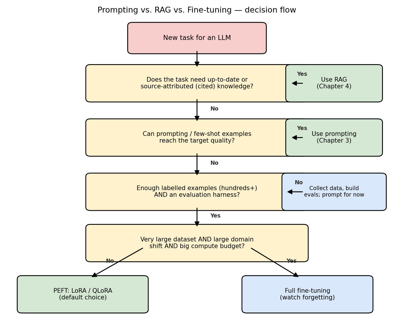
Decision criteria as a table (exam-friendly form):
| Criterion | Prompting | Retrieval-augmented generation | Fine-tuning |
|---|---|---|---|
| Knowledge freshness needed | poor | best (index is updatable) | poor (frozen at training) |
| Source attribution / citations | no | yes | no |
| Persistent style / format | weak | weak | best |
| Labelled data required | none–few | none (documents instead) | hundreds+ |
| Per-request cost | high (long prompts) | medium (retrieval + tokens) | low (short prompts) |
| Up-front cost | none | index build | training run |
| Risk of capability damage | none | none | catastrophic forgetting |
Rule of thumb from the lecture: fine-tune for behavior, retrieve for knowledge, prompt for quick experiments. The three combine: a fine-tuned model can still use retrieval and good prompts.
Code example: deciding if fine-tuning is appropriate
def choose_adaptation(num_examples, knowledge_freshness_days, needs_citations, eval_harness):
    if needs_citations or knowledge_freshness_days < 30:
        return "Use retrieval-augmented generation"
    if num_examples < 100:
        return "Use few-shot prompting"
    if not eval_harness:
        return "Build an evaluation harness first"
    return "Fine-tune (parameter-efficient first)"

print(choose_adaptation(500, 365, False, True))   # -> Fine-tune (parameter-efficient first)
বাংলা ব্যাখ্যা: সিদ্ধান্তের সূত্রটা এক লাইনে: আচরণ শেখাতে ফাইন-টিউন, তাজা তথ্যের জন্য RAG, দ্রুত পরীক্ষার জন্য প্রম্পট। ডেটা প্রতিদিন বদলালে বা সূত্র (citation) দেখাতে হলে RAG-ই একমাত্র সঠিক উত্তর, কারণ ওজনের ভেতরের জ্ঞান আপডেটও করা যায় না, দেখানোও যায় না। আর ইভ্যালুয়েশন ছাড়া ফাইন-টিউন করা মানে চোখ বেঁধে অপারেশন করা।
6.2 Full Fine-tuning
6.2.1 Definition and loss
Full fine-tuning updates every parameter \(\theta\) of the base model by minimizing the task loss (negative log-likelihood) on the fine-tuning dataset:
Optionally with a regularization term that pulls the solution back toward the pretrained weights:
| Symbol | Meaning |
|---|---|
| \(\theta\) | all model parameters (trainable) |
| \(\theta_{pretrained}\) | frozen snapshot of the parameters before fine-tuning |
| \(L_{task}\) | cross-entropy on the fine-tuning data |
| \(\lambda\) | regularization strength (how hard we pull back to the pretrained point) |
| \((x, y)\) | input and target sequence pair |
বাংলা ব্যাখ্যা: দ্বিতীয় সূত্রটা গুরুত্বপূর্ণ — \(\lambda\) যত বড়, মডেল তত কম দূরে সরতে পারে প্রি-ট্রেইনড অবস্থান থেকে, ফলে ভুলে যাওয়া (forgetting) তত কম, কিন্তু নতুন কাজ শেখাও তত সীমিত। এটাই regularization-এর দৃষ্টিতে forgetting নিয়ন্ত্রণ।
6.2.2 Catastrophic forgetting — cause, mechanism, consequence
- Cause: the fine-tuning dataset covers only a narrow slice of the pretraining distribution.
- Mechanism: gradient descent moves all weights to reduce loss on that slice; weights that encoded unrelated capabilities are overwritten because nothing in the new loss protects them (the optimizer has no memory of the old data).
- Consequence: general capabilities (reasoning, other languages, world knowledge) measurably degrade, even though task performance improves.
Regularization view. The penalty \((\lambda/2)\,\|\theta - \theta_{pretrained}\|^2\) treats the pretrained point as a prior: deviations are taxed quadratically. More refined versions (elastic weight consolidation) weight each coordinate by its estimated importance \(F_i\) for old capabilities:
Parameter-efficient methods take this idea to the limit: instead of taxing deviation, they structurally constrain it — Low-Rank Adaptation only permits updates inside a rank-\(r\) subspace and the base stays exactly frozen.
বাংলা ব্যাখ্যা: ভুলে যাওয়ার কারণটা বোঝো: নতুন লস ফাংশন শুধু নতুন ডেটার পারফরম্যান্স দেখে — পুরোনো দক্ষতা রক্ষার কোনো শর্ত তাতে নেই, তাই গ্রেডিয়েন্ট নির্দ্বিধায় পুরোনো জ্ঞানের ওজনগুলো মুছে নতুন কাজে লাগায়। LoRA-তে বেস একদম জমাট (frozen) থাকে বলে ক্ষতিটা কাঠামোগতভাবেই সীমিত — আর অ্যাডাপ্টার খুলে ফেললে আদি মডেল হুবহু ফিরে আসে।
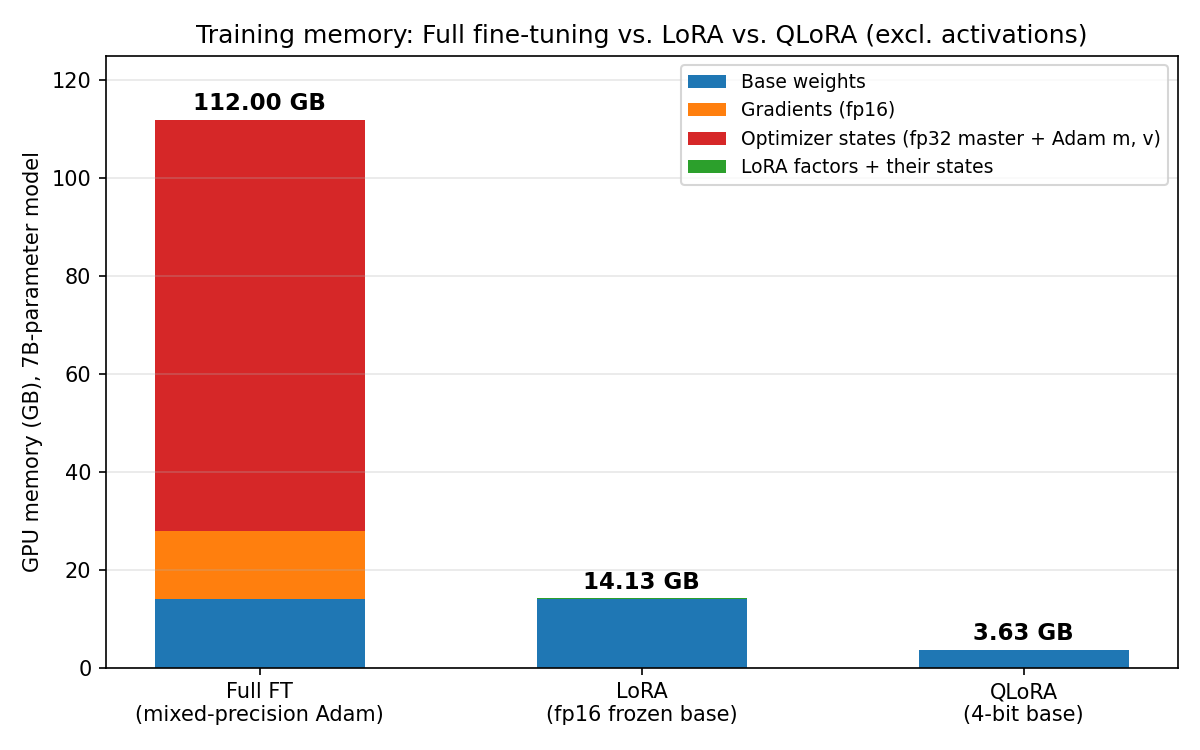
6.2.3 Training-memory arithmetic (the famous 16 bytes per parameter)
Mixed-precision training with the Adam optimizer keeps, per parameter:
| Component | Precision | Bytes per parameter |
|---|---|---|
| Working weights | 16-bit float | 2 |
| Gradients | 16-bit float | 2 |
| Master copy of weights | 32-bit float | 4 |
| Adam first moment \(m\) | 32-bit float | 4 |
| Adam second moment \(v\) | 32-bit float | 4 |
| Total | 16 |
Worked example (7B model, full fine-tuning).
Memory = 7 × 10⁹ parameters × 16 bytes/parameter
       = 112 × 10⁹ bytes
       = 112.00 GB        (plus activations, which depend on batch size and sequence length)
No single commodity GPU (24–80 GB) holds this; full fine-tuning of a 7B model requires multi-GPU sharding.
Comparison preview (details in 6.3):
| Setting | Base weights | Trainable states | Approx. total (excl. activations) |
|---|---|---|---|
| Full fine-tuning 7B | 14.00 GB (16-bit, inside the 112) | 112.00 GB total | 112.00 GB |
| Low-Rank Adaptation, \(r=8\) | 14.00 GB frozen 16-bit | 8,388,608 × 16 B = 134.22 MB ≈ 0.13 GB | ≈ 14.13 GB |
| QLoRA, \(r=8\) | 3.50 GB frozen 4-bit | ≈ 0.13 GB | ≈ 3.63 GB |
বাংলা ব্যাখ্যা: ১৬ বাইট/প্যারামিটার সংখ্যাটা মুখস্থ রাখো আর ভাঙতে শেখো: ২ (ওজন fp16) + ২ (গ্রেডিয়েন্ট fp16) + ৪ (মাস্টার ওজন fp32) + ৪ (Adam-এর প্রথম মোমেন্ট) + ৪ (দ্বিতীয় মোমেন্ট)। গুণ করলেই ৭B × ১৬ = ১১২ GB। LoRA-তে বেসের জন্য শুধু ২ বাইট (forward-এর ওজন) লাগে — গ্রেডিয়েন্ট আর অপটিমাইজার স্টেট লাগে কেবল ক্ষুদ্র অ্যাডাপ্টারের জন্য। এই ভাঙানোটাই পরীক্ষার ৫-নম্বরী অঙ্ক।
6.2.4 When full fine-tuning is still the right tool
- Very large fine-tuning datasets (millions of examples) and a strong domain shift (e.g., training a code-specialized model from a general base).
- When the highest possible task quality justifies cluster-scale compute and a careful forgetting-mitigation recipe (data mixing with pretraining-like data, small learning rate, early stopping).
Code example: full fine-tuning loop (toy scale — a 7B model will not fit on a laptop)
import torch, torch.nn as nn, torch.nn.functional as F
torch.manual_seed(0)

class Toy(nn.Module):                      # stands in for an LLM
    def __init__(self, V=50, d=64):
        super().__init__()
        self.emb = nn.Embedding(V, d)
        self.lin = nn.Linear(d, V)
    def forward(self, x): return self.lin(self.emb(x))

model = Toy()
opt = torch.optim.AdamW(model.parameters(), lr=1e-3)   # ALL parameters trainable
data = torch.randint(0, 50, (256, 8))
for step in range(50):
    x, y = data[:, :-1], data[:, 1:]
    loss = F.cross_entropy(model(x).reshape(-1, 50), y.reshape(-1))
    opt.zero_grad(); loss.backward(); opt.step()
print("Final loss:", loss.item())
বাংলা ব্যাখ্যা: Full fine-tuning এখনো দরকার হয় যখন ডেটা বিশাল আর ডোমেইন একেবারে আলাদা — যেমন সাধারণ মডেল থেকে কোডিং-বিশেষজ্ঞ মডেল বানানো। কিন্তু ডিফল্ট পছন্দ সবসময় PEFT; full fine-tuning হলো শেষ অস্ত্র, প্রথম নয়।
6.3 Parameter-Efficient Fine-Tuning (PEFT)
The core idea: freeze the base model, train a tiny number of new parameters. This section is the mathematical heart of the chapter.
6.3.1 Matrix rank — recap with a worked example
Definition. The rank of a matrix is the number of linearly independent rows (equivalently, columns). A matrix \(M \in \mathbb{R}^{d \times k}\) that factors as an outer product of two vectors has rank 1; a product of an \(d \times r\) and an \(r \times k\) matrix has rank at most \(r\).
Worked 2×2 rank-1 example (outer product). Take
Check the rank: - Row 2 = 0.50 × Row 1 → the rows are linearly dependent. - Determinant: \(6 \cdot (-1) - (-2) \cdot 3 = -6.00 + 6.00 = 0.00\) → not full rank. - Exactly one independent row → rank 1.
Storage view: the full matrix has \(2 \times 2 = 4\) entries; the factors have \(2 + 2 = 4\) entries — no saving at this toy size. But for \(d = k = 4096\) and rank 8 the factors need \(r(d+k) = 65{,}536\) numbers instead of \(dk = 16{,}777{,}216\). The saving grows with matrix size, which is exactly why this matters for LLMs.
Why is the fine-tuning update \(\Delta W\) approximately low-rank? - Empirical: Aghajanyan et al. (2020) showed fine-tuning objectives can be optimized inside a surprisingly low-dimensional reparametrization — the task's intrinsic dimension is small (often hundreds, not millions, of directions for large pretrained models). - Intuition: the pretrained model already contains the needed features; adaptation mostly re-combines and re-weights existing directions rather than learning new ones. The singular-value spectrum of the ideal \(\Delta W\) decays fast, so a rank-\(r\) truncation (best possible by the Eckart–Young theorem) captures most of the useful update. - Consequence: restricting the update to rank \(r \ll \min(d,k)\) loses little quality but saves enormous memory — the founding hypothesis of Low-Rank Adaptation.
import numpy as np
np.random.seed(0)
A = np.random.randn(4, 3); B = np.random.randn(3, 5)
M = A @ B                       # shape 4x5, but rank ≤ 3
print("rank(M) =", np.linalg.matrix_rank(M))   # -> 3
বাংলা ব্যাখ্যা: Rank মানে ম্যাট্রিক্সে আসলে কতগুলো স্বাধীন দিক (direction) আছে। ২×২ উদাহরণে দ্বিতীয় সারিটা প্রথম সারির অর্ধেক — তাই তথ্য আসলে একটাই দিকের, rank = 1। ফাইন-টিউনিংয়ের আপডেটও এমন: বিশাল ম্যাট্রিক্স দেখালেও কাজের পরিবর্তন ক'টা মাত্র দিকে ঘটে, কারণ দরকারি ফিচারগুলো প্রি-ট্রেইনিংয়েই শেখা হয়ে গেছে — নতুন কাজ শুধু সেগুলোর নতুন মিশ্রণ চায়।
6.3.2 Low-Rank Adaptation (LoRA)
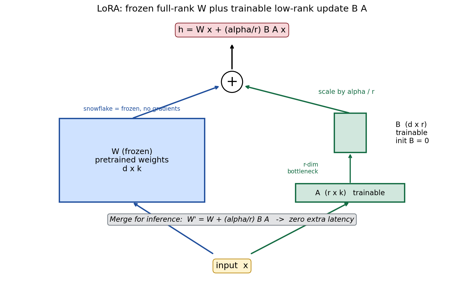
Formulation. A frozen pretrained weight matrix \(W \in \mathbb{R}^{d \times k}\) is augmented by a trainable low-rank update:
with shapes \(A \in \mathbb{R}^{r \times k}\), \(B \in \mathbb{R}^{d \times r}\) and \(r \ll \min(d, k)\).
| Symbol | Meaning | Trainable? |
|---|---|---|
| \(W \in \mathbb{R}^{d \times k}\) | pretrained weight matrix (e.g., a query projection) | no — frozen |
| \(A \in \mathbb{R}^{r \times k}\) | "down" factor; initialized random Gaussian | yes |
| \(B \in \mathbb{R}^{d \times r}\) | "up" factor; initialized to all zeros | yes |
| \(r\) | rank of the update — capacity hyperparameter | hyperparameter |
| \(\alpha\) | scaling factor — effective update is \((\alpha/r)BA\) | hyperparameter |
| \(d, k\) | output and input dimension of the layer | architecture |
Key design choices: - Initialization: \(A \sim \mathcal{N}(0, \sigma^2)\), \(B = 0\). Then \(\Delta W = BA = 0\) at the start, so training begins exactly at the pretrained model — no random disturbance of base behavior. - Scaling \(\alpha/r\): decouples the update magnitude from the rank. If you double \(r\), the per-direction contribution halves, keeping the overall scale comparable. \(r\) controls capacity (how many directions can change); \(\alpha\) controls effective step size. They are not redundant. - Forward pass: \(y = Wx + (\alpha/r)\,B(Ax)\) — computed as two skinny matrix multiplications during training. - Merging for inference: compute \(W' = W + (\alpha/r)BA\) once; thereafter a single dense multiplication, i.e., zero added latency compared with the base model.
Worked example 1 — square attention projection. \(d = k = 4096\), \(r = 8\):
LoRA trainable:  r(d + k) = 8 × (4096 + 4096) = 8 × 8192 = 65,536
Full matrix:     d · k    = 4096 × 4096        = 16,777,216
Reduction:       16,777,216 / 65,536           = 256.00×
Trainable share: 65,536 / 16,777,216 × 100     = 0.39 %
Worked example 2 — non-square feed-forward projection. The feed-forward up-projection of a 7B-class model maps 4096 → 11008, so \(W \in \mathbb{R}^{11008 \times 4096}\) (\(d = 11008\), \(k = 4096\)), choose \(r = 16\):
LoRA trainable:  r(d + k) = 16 × (11008 + 4096) = 16 × 15,104 = 241,664
Full matrix:     d · k    = 11008 × 4096         = 45,088,768
Reduction:       45,088,768 / 241,664            = 186.58×
Trainable share: 241,664 / 45,088,768 × 100      = 0.54 %
Note how the reduction factor depends on shape: \(\frac{dk}{r(d+k)}\) — bigger and squarer matrices give bigger savings at fixed \(r\).
Pros - Tiny trainable footprint (megabytes); the "LoRA file" ships separately from the base. - Many adapters per base model — one per task or per customer; hot-swappable at inference. - Merged inference adds zero latency. - Base frozen → low risk of catastrophic forgetting; removing the adapter restores the original model exactly.
Cons - Slightly below full fine-tuning quality on very large datasets / strong domain shifts. - Two extra hyperparameters (\(r\), \(\alpha\)) plus the choice of target matrices.
বাংলা ব্যাখ্যা: LoRA-র পুরো গল্প একটা সূত্রে: \(W' = W + (\alpha/r)BA\)। বিশাল \(W\) জমাট, শেখে শুধু দুই চিকন ম্যাট্রিক্স \(B\) (লম্বা×\(r\)) আর \(A\) (\(r\)×চওড়া)। \(B=0\) দিয়ে শুরু — তাই প্রথম স্টেপে মডেল হুবহু আগের মতোই। হিসাবের কৌশল: trainable = \(r(d+k)\), পুরো ম্যাট্রিক্স = \(dk\); ভাগ করলেই কত গুণ সাশ্রয় বেরিয়ে আসে (৪০৯৬-বর্গে \(r=8\) দিলে ঠিক ২৫৬ গুণ)।
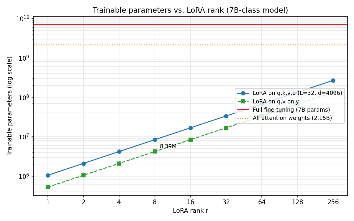
6.3.3 Total LoRA parameters across a whole model (worked sum)
Attach LoRA with \(r = 8\) to the four attention projections (query, key, value, output), each \(4096 \times 4096\), in all \(L = 32\) layers of a 7B-class model:
Per matrix:  r(d + k)        = 8 × 8192            = 65,536
Per layer:   4 × 65,536      (q, k, v, o)          = 262,144
Total:       32 × 262,144                          = 8,388,608  ≈ 8.39 M

Share of base: 8,388,608 / 7,000,000,000 × 100     = 0.12 %
General formula for \(L\) layers, a set \(T\) of target matrices with shapes \((d_t, k_t)\):
Extension check (matches the Level-5 coding task below): adding the three feed-forward matrices (gate 11008×4096, up 11008×4096, down 4096×11008) at \(r=8\) gives
Per layer FFN part: 8 × (15,104 + 15,104 + 15,104) = 8 × 45,312 = 362,496
Total all targets:  32 × (262,144 + 362,496) / 32 … = 32 × 624,640 = 19,988,480 ≈ 19.99 M  (0.29 % of 7B)
বাংলা ব্যাখ্যা: মোট প্যারামিটার গোনার ছক: (এক ম্যাট্রিক্সে \(r(d+k)\)) × (প্রতি লেয়ারে কয়টা ম্যাট্রিক্স) × (কয়টা লেয়ার)। ৩২ লেয়ার × ৪ ম্যাট্রিক্স × ৬৫,৫৩৬ = ৮৩,৮৮,৬০৮ — মানে ৭ বিলিয়নের মাত্র ০.১২%। পরীক্ষায় ধাপে ধাপে লিখো: আগে এক ম্যাট্রিক্স, তারপর এক লেয়ার, তারপর গোটা মডেল — মাঝপথে গুণ ভুল হলে আংশিক নম্বর তবু থাকবে।
6.3.4 Adapters (bottleneck modules)
Formulation. Insert a small residual bottleneck multilayer perceptron after each transformer sub-layer:
| Symbol | Shape | Meaning |
|---|---|---|
| \(W_{down}\) | \(r \times d\) | down-projection into the bottleneck |
| \(W_{up}\) | \(d \times r\) | up-projection back to model width |
| \(r\) | scalar | bottleneck width (plays the same capacity role as the LoRA rank) |
| \(x, y\) | \(d\) | sub-layer input / output (residual connection keeps identity path) |
Parameter count per adapter module ≈ \(2dr\) for the two weight matrices, plus biases (\(r + d\)):
Worked example. \(d = 4096\), \(r = 8\):
Weights: 2 · d · r = 2 × 4096 × 8       = 65,536
Biases:  r + d     = 8 + 4096           = 4,104
Per module:                               69,640
Per layer (2 modules: after attention and after feed-forward): 2 × 69,640 = 139,280
Whole model (L = 32):  32 × 139,280     = 4,456,960 ≈ 4.46 M
Comparison with LoRA (same \(d = 4096\), \(r = 8\), \(L = 32\)):
| Property | Adapters (Houlsby) | Low-Rank Adaptation |
|---|---|---|
| Trainable parameters (this config) | ≈ 4.46 M | ≈ 8.39 M (q,k,v,o) |
| Where it lives | new sequential module in the layer | parallel additive update to existing matrices |
| Nonlinearity | yes (GELU in the bottleneck) | no (purely linear update) |
| Inference latency | adds an extra sequential computation per layer — cannot be merged (because of the nonlinearity) | zero after merging \(W' = W + (\alpha/r)BA\) |
| Restore base model | remove modules | remove/unmerge factors |
The latency argument is a classic exam question: the adapter's GELU makes it impossible to fold the module into the neighboring weight matrix, whereas the LoRA update is linear in \(x\) and therefore mergeable.
বাংলা ব্যাখ্যা: অ্যাডাপ্টার হলো লেয়ারের ভেতরে বসানো ছোট "টোলপ্লাজা" — ইনপুট সরু হয়ে (\(d{\to}r\)) আবার চওড়া হয় (\(r{\to}d\)), মাঝে GELU। ওই nonlinearity-র কারণেই একে মূল ওজনে মেশানো যায় না, তাই প্রতি ইনফারেন্সে বাড়তি সময় লাগে। LoRA-র আপডেট পুরোপুরি রৈখিক, তাই মেশানো যায় — latency শূন্য। এই এক লাইনের তুলনাটাই ৩-নম্বরী "Explain why" প্রশ্নের প্রাণ।
6.3.5 Quantization and affine quantization (the Q in QLoRA)
Idea. Store each weight with \(b\) bits instead of 16. Affine (asymmetric) quantization maps the real interval \([x_{min}, x_{max}]\) onto the integers \(\{0, \dots, 2^b - 1\}\):
scale:       s = (x_max − x_min) / (2^b − 1)
zero-point:  z = round(−x_min / s)
quantize:    q = clamp( round(x / s) + z , 0 , 2^b − 1 )
dequantize:  x̂ = s · (q − z)
| Symbol | Meaning |
|---|---|
| \(b\) | bit width (8 → 256 levels, 4 → 16 levels) |
| \(s\) | scale: real-value width of one integer step |
| \(z\) | zero-point: which integer represents the real value 0 |
| \(q\) | stored integer code |
| \(\hat{x}\) | reconstructed (dequantized) value; $ |
Worked example (\(b = 4\)). Weights lie in \([-2.00, 1.00]\):
s = (1.00 − (−2.00)) / (2⁴ − 1) = 3.00 / 15 = 0.20
z = round(2.00 / 0.20) = round(10.00) = 10

Quantize x = 0.57:
  x / s = 0.57 / 0.20 = 2.85  → round = 3
  q = 3 + 10 = 13               (inside [0, 15] ✓)

Dequantize:
  x̂ = 0.20 × (13 − 10) = 0.60

Rounding error: |0.60 − 0.57| = 0.03      (≤ s/2 = 0.10 ✓)
Storage per parameter: 16-bit float = 2 bytes; 8-bit = 1 byte; 4-bit = 0.5 bytes. QLoRA uses a 4-bit data type designed for normally-distributed weights (NormalFloat4) plus double quantization of the per-block scales to shave the overhead further.
বাংলা ব্যাখ্যা: কোয়ান্টাইজেশন মানে ওজনগুলোকে মোটা দাগের স্কেলে মাপা — পুরো রেঞ্জকে \(2^b\)টা ধাপে ভাগ করা হয়; \(s\) হলো এক ধাপের দৈর্ঘ্য, \(z\) বলে দেয় শূন্য কোন ধাপে পড়ে। ধাপ যত মোটা, ভুল তত বেশি — সর্বোচ্চ ভুল \(s/2\)। হিসাবের ক্রমটা মুখস্থ: \(s\) → \(z\) → \(q\) → \(\hat{x}\) → error; পরীক্ষায় এই পাঁচ ধাপই পাঁচ নম্বর।
6.3.6 QLoRA = 4-bit frozen base + 16-bit LoRA factors
Recipe (Dettmers et al. 2023): 1. Quantize the frozen base model to 4 bits (NormalFloat4, double quantization). 2. Attach LoRA factors \(A, B\) kept in 16-bit precision; only these receive gradients. 3. Backpropagate through the dequantized 4-bit weights into the LoRA factors. 4. Use a paged optimizer to survive memory spikes.
Memory arithmetic, 7B model, \(r = 8\) on q,k,v,o:
Full fine-tuning:   7 × 10⁹ × 16 B               = 112.00 GB
LoRA (fp16 base):   7 × 10⁹ × 2 B  + 8,388,608 × 16 B = 14.00 GB + 0.13 GB ≈ 14.13 GB
QLoRA (4-bit base): 7 × 10⁹ × 0.5 B + 8,388,608 × 16 B =  3.50 GB + 0.13 GB ≈  3.63 GB
(The trainable-side 16 B/parameter = 2 weight + 2 gradient + 12 optimizer, same accounting as in 6.2.3; activations come on top in all three cases.) QLoRA famously enables fine-tuning a 65B model on a single 48 GB graphics card: \(65 \times 10^9 \times 0.5\,B = 32.50\) GB for the base, leaving room for adapters and activations.
Trade-off: each forward pass dequantizes blocks of weights on the fly → some extra compute per step, in exchange for the ~4× memory cut versus a 16-bit base.
বাংলা ব্যাখ্যা: QLoRA-র সমীকরণ: জমাট বেস ৪-বিটে (প্যারামিটার-প্রতি মাত্র আধা বাইট) + ছোট LoRA ফ্যাক্টর ১৬-বিটে। ৭B মডেল: ১১২ GB → ১৪.১৩ GB → ৩.৬৩ GB — এই তিনটা সংখ্যার সিঁড়িটা মনে রাখো। দাম দিতে হয় গতিতে: প্রতি স্টেপে ওজন ডিকোয়ান্টাইজ করতে হয়, তাই একটু ধীর — কিন্তু ৬৫B মডেল একটা মাত্র GPU-তে টিউন করা যায়, এটাই বিপ্লব।
6.3.7 Code: Low-Rank Adaptation from scratch on a single linear layer
import torch, torch.nn as nn

class LoRALinear(nn.Module):
    def __init__(self, base: nn.Linear, r=8, alpha=16):
        super().__init__()
        self.base = base
        for p in base.parameters(): p.requires_grad_(False)   # freeze W (and bias)
        d_out, d_in = base.weight.shape
        self.A = nn.Parameter(torch.randn(r, d_in) * 0.01)    # A ~ N(0, σ²)
        self.B = nn.Parameter(torch.zeros(d_out, r))          # B = 0  → ΔW = 0 at start
        self.scale = alpha / r
    def forward(self, x):
        return self.base(x) + (x @ self.A.T) @ self.B.T * self.scale

torch.manual_seed(0)
base = nn.Linear(64, 64)
lora = LoRALinear(base, r=4)
x = torch.randn(2, 64)
print("output shape:", lora(x).shape)                                     # (2, 64)
print("trainable:", sum(p.numel() for p in lora.parameters() if p.requires_grad))  # 4*(64+64)=512
print("frozen base:", sum(p.numel() for p in lora.base.parameters()))     # 64*64+64 = 4160
Sanity checks worth memorizing: trainable \(= r(d_{in} + d_{out}) = 4 \times 128 = 512\); before any training step the output equals the base output exactly (because \(B = 0\)).
Library version (Hugging Face peft):
# from peft import LoraConfig, get_peft_model
# from transformers import AutoModelForCausalLM
# base  = AutoModelForCausalLM.from_pretrained("meta-llama/Llama-3.1-8B")
# cfg   = LoraConfig(r=8, lora_alpha=16,
#                    target_modules=["q_proj", "k_proj", "v_proj", "o_proj"])
# model = get_peft_model(base, cfg)
# model.print_trainable_parameters()    # ~0.1 % trainable
If print_trainable_parameters() reports 0.42 % trainable: that is the share of parameters with requires_grad=True. For LoRA on \(L\) target matrices it is \(L \cdot r(d+k)\) divided by the total parameter count; increasing \(r\) increases both capacity and this percentage proportionally.
বাংলা ব্যাখ্যা: কোডের তিনটা জায়গা খেয়াল করো: (১) বেসের সব প্যারামিটার requires_grad_(False) — জমাট; (২) \(A\) র্যান্ডম কিন্তু \(B\) শূন্য — তাই শুরুতে আউটপুট অবিকল বেসের মতো; (৩) forward-এ আগে \(Ax\) (সরু), পরে \(B(\cdot)\) — কখনোই পুরো \(BA\) ম্যাট্রিক্স ট্রেনিংয়ে বানানো হয় না, এতেই গতি। print_trainable_parameters() দিয়ে সবসময় যাচাই করো সত্যিই অল্প প্যারামিটার শিখছে কি না।
Algorithms in This Chapter
Algorithm A — LoRA forward pass
input x
y_base = W x                       # frozen
y_lora = (α/r) · B (A x)           # two skinny multiplications
y      = y_base + y_lora
Algorithm B — LoRA merge for deployment
W_merged = W + (α/r) · B A          # done once, offline
serve with W_merged                  # zero added latency
(unmerge: W = W_merged − (α/r) · B A  restores the base exactly)
Algorithm C — Full fine-tuning step
loss ← cross_entropy(model(x), y)
zero gradients; loss.backward(); optimizer.step()     # touches ALL parameters
Algorithm D — QLoRA training step
forward: dequantize 4-bit base blocks on the fly; add (α/r)·B(Ax) in 16-bit
loss in 16-bit
backward: gradients flow ONLY into A and B
optimizer step on A, B (paged Adam)
বাংলা ব্যাখ্যা: চারটা অ্যালগরিদমের পার্থক্য এক নজরে: A হলো ট্রেনিংয়ের forward (দুটো চিকন গুণ), B হলো ডিপ্লয়মেন্টের কৌশল (একবার মিশিয়ে নিলে আর খরচ নেই, আবার বিয়োগ করলে বেস ফেরত), C-তে গ্রেডিয়েন্ট সব ওজনে যায়, D-তে শুধু \(A, B\)-তে। পরীক্ষায় pseudocode চাইলে এগুলোই লিখবে।
Real-Life Applications
| Use case | Recommended approach | Why |
|---|---|---|
| Format every output as JSON | Low-Rank Adaptation + supervised fine-tuning | persistent format adoption |
| Adopt company tone-of-voice | Low-Rank Adaptation + supervised fine-tuning | persistent style |
| Answer with today's stock prices | retrieval-augmented generation (not fine-tuning) | knowledge changes daily |
| Classify medical reports | Low-Rank Adaptation on a domain dataset | small labelled dataset, stable domain |
| Instruction-tune a raw base model | full or LoRA supervised fine-tuning | broad behavior change |
| Align to safety preferences | preference alignment (Chapter 2.10) | preference optimization, not task loss |
| Coding assistant from a general base | full fine-tuning (large data, big shift) + preference tuning | domain shift too large for tiny updates |
| One adapter per enterprise customer | LoRA hot-swapping on a shared base | megabyte adapters, per-tenant isolation |
Limits: fine-tuning is not a substitute for retrieval when knowledge is volatile, and not a substitute for alignment when safety preferences are the goal.
বাংলা ব্যাখ্যা: বাস্তব প্রয়োগ মুখস্থ নয়, প্যাটার্নটা ধরো: স্টাইল/ফরম্যাট/ডোমেইন-আচরণ → ফাইন-টিউনিং; তাজা/উদ্ধৃতিযোগ্য তথ্য → RAG; নিরাপত্তা-পছন্দ → অ্যালাইনমেন্ট। মাল্টি-টেন্যান্ট SaaS-এর কেসটা বিশেষ সুন্দর — এক বেস মডেল, প্রতি গ্রাহকের জন্য কয়েক মেগাবাইটের আলাদা LoRA ফাইল, অনুরোধ অনুযায়ী লাগানো-খোলা যায়।
Exam-Focused Summary
| Topic | Memorize |
|---|---|
| When to fine-tune | persistent style/behavior, hundreds+ examples, evaluation harness ready |
| When NOT to | volatile facts (→ retrieval), tiny data (→ prompting), no evaluation, citations needed |
| LoRA update | \(W' = W + (\alpha/r)BA\), \(A \in \mathbb{R}^{r \times k}\) random, \(B \in \mathbb{R}^{d \times r}\) zero-init |
| LoRA trainable per matrix | \(r(d+k)\) vs. full \(dk\); reduction \(= dk / r(d+k)\) |
| Worked anchor numbers | 4096², r=8 → 65,536 vs 16,777,216 → 256.00×; whole 7B q,k,v,o, L=32 → 8,388,608 (0.12 %) |
| Adapter | \(y = x + W_{up}\,\mathrm{GELU}(W_{down}\,x)\); ≈ \(2dr\) + biases; adds latency (GELU blocks merging) |
| Bytes per parameter (training, Adam mixed precision) | 2 + 2 + 4 + 4 + 4 = 16 → 7B: 112.00 GB |
| Memory ladder 7B | full 112.00 GB → LoRA ≈ 14.13 GB → QLoRA ≈ 3.63 GB |
| Affine quantization | \(s = (x_{max} - x_{min})/(2^b - 1)\); \(z = \mathrm{round}(-x_{min}/s)\); error ≤ \(s/2\) |
| QLoRA | 4-bit NormalFloat frozen base (0.5 B/param) + 16-bit LoRA factors + paged optimizer |
| Catastrophic forgetting | narrow loss overwrites unprotected weights; mitigations: penalty toward \(\theta_{pretrained}\), data mixing, freezing (PEFT) |
বাংলা ব্যাখ্যা: রিভিশনের সময় এই টেবিলের "anchor" সংখ্যাগুলো বারবার হাতে কষো: ২৫৬×, ৮৩,৮৮,৬০৮, ০.১২%, ১৬ বাইট, ১১২ GB, ৩.৬৩ GB, error ≤ \(s/2\)। পরীক্ষার হলে নতুন সংখ্যা দিলেও পদ্ধতি একই থাকবে — শুধু \(d, k, r, L\) বদলে যাবে।
Common Traps (lose-a-point list)
- Confusing fine-tuning with retrieval-augmented generation — weights store behavior, the index stores facts.
- Forgetting the \((\alpha/r)\) scaling when computing the merged weight or gradients.
- Computing LoRA parameters as \(r \cdot d \cdot k\) instead of \(r(d+k)\).
- Using 1 GB = 2³⁰ bytes in one line and 10⁹ bytes in the next — pick one (the lecture uses 10⁹) and state it.
- Claiming adapters can be merged — the GELU nonlinearity prevents it; only the linear LoRA update merges.
- Forgetting to freeze the base model — then it is just full fine-tuning with extra parameters.
- Treating supervised fine-tuning alone as alignment — preference optimization is still needed for safety.
- Choosing \(r\) too small (underfits the task) or needlessly large (memory, more drift from base, overfitting risk).
বাংলা ব্যাখ্যা: সবচেয়ে দামি দুটো ভুল: \(r(d+k)\)-র জায়গায় \(r \cdot d \cdot k\) লেখা, আর \((\alpha/r)\) স্কেলিং ভুলে যাওয়া — দুটোতেই পুরো অঙ্ক ভেস্তে যায়। আর মনে রাখো: অ্যাডাপ্টার মেশানো যায় না (GELU আছে বলে), LoRA যায় (রৈখিক বলে) — উল্টে বললে নম্বর কাটা নিশ্চিত।
Mock Exam — Chapter 6
Instructions: 120 minutes for the full exam; this chapter block is worth 50 points. Use the technical terms from the lecture. Do not use abbreviations. A non-programmable calculator is allowed. Round all numerical results to 2 decimals unless stated otherwise.
Level 1 — Basic (10 points)
Q1.1 (1 pt). Which statement best describes parameter-efficient fine-tuning? - (a) It updates all parameters of the base model but with a smaller learning rate. - (b) It freezes the base model and trains only a small number of (often newly added) parameters. - (c) It compresses the base model to fewer bits so it fits on one graphics card. - (d) It replaces gradient updates entirely with in-context examples.
Q1.2 (1 pt). Which statement best describes the role of the rank \(r\) in Low-Rank Adaptation? - (a) It sets the number of transformer layers that receive an update. - (b) It sets the numerical precision of the trainable factors. - (c) It sets the number of independent directions in which the weight matrix can change, and thereby the trainable-parameter count \(r(d+k)\). - (d) It sets the learning rate of the adapter optimizer.
Q1.3 (1 pt). Which statement best describes QLoRA? - (a) The base model is quantized to 4 bits and also trained in 4 bits. - (b) The Low-Rank Adaptation factors are quantized to 4 bits while the base stays in 16 bits. - (c) The frozen base model is stored in 4 bits while 16-bit Low-Rank Adaptation factors are trained on top. - (d) The optimizer states are quantized to 4 bits while everything else stays in 16 bits.
Q1.4 (1 pt). Which statement best describes why a merged Low-Rank Adaptation model has the same inference latency as the base model? - (a) The adapter is executed on a second graphics card in parallel. - (b) The update \((\alpha/r)BA\) is folded into the weight once, so inference performs the same single matrix multiplication as before. - (c) The rank \(r\) is so small that the extra computation takes no measurable time. - (d) The factors are cached in fast memory after the first request.
Q1.5 (3 pts). Define parameter-efficient fine-tuning and rank precisely, using the technical terms from the lecture.
Q1.6 (3 pts). Define QLoRA and catastrophic forgetting precisely, using the technical terms from the lecture.
Level 2 — Intuitive "Explain why" (9 points, 3 each; structure each answer as cause → mechanism → consequence)
Q2.1. Explain why a low-rank update is usually sufficient to adapt a large pretrained language model to a new task.
Q2.2. Explain why a merged Low-Rank Adaptation adds zero inference latency, while an adapter module always adds latency.
Q2.3. Explain why full fine-tuning suffers more from catastrophic forgetting than Low-Rank Adaptation.
Level 3 — Numerical (15 points, 5 each; show every step, 2 decimals)
Q3.1. A 7B-class model has \(L = 32\) transformer layers with query/key/value/output projections of size \(4096 \times 4096\). Low-Rank Adaptation with rank \(r = 16\) is attached to the query and value projections only. (a) Trainable parameters per matrix, per layer, and for the whole model. (b) Reduction factor versus fully training one \(4096 \times 4096\) matrix. (c) Trainable share of the 7,000,000,000-parameter base in percent.
Q3.2. You have a single 24 GB graphics card and a 13B-parameter model (\(L = 40\) layers, hidden size 5120). Decide which of the following fits, using 1 GB = \(10^9\) bytes and ignoring activations (state this assumption): (a) full fine-tuning with mixed-precision Adam (16 bytes per parameter), (b) Low-Rank Adaptation (\(r = 8\) on query/key/value/output) with a 16-bit frozen base, (c) QLoRA (4-bit frozen base) with the same adapters. For (b) and (c), compute the adapter parameter count and its training-state memory at 16 bytes per trainable parameter.
Q3.3. Affine quantization with \(b = 4\) bits over the weight range \([-1.00, 2.00]\). (a) Compute the scale \(s\) and the zero-point \(z\). (b) Quantize \(x = -0.47\) (give the integer code). (c) Dequantize and state the absolute rounding error. (d) State the maximum possible rounding error of this quantizer.
Level 4 — Transfer / TU-hard mini-cases (10 points; 5 + 5; name the technique, justify, give the trade-off)
Q4.1 (5 pts). A company has two separately trained Low-Rank Adaptation adapters on the same frozen base: one for legal tone, one for strict JSON output. An engineer proposes serving both at once by simply adding the updates: \(W' = W + \Delta W_{legal} + \Delta W_{JSON}\). Assess this proposal: when does such "task arithmetic" work, what is the interference risk, and name two safer alternatives with their trade-offs.
Q4.2 (5 pts). (Choose ONE of the two scenarios; both are graded equally.) (i) Rank versus intrinsic dimension. A team raises the rank from \(r = 8\) to \(r = 256\) hoping for better quality. Task accuracy barely moves, but held-out general-capability scores drop and memory rises. Explain using the concept of intrinsic dimension, and give a recommendation. (ii) When retrieval strictly dominates. A bank's chatbot must answer from regulations that change weekly, must cite the exact source paragraph, and must respect per-user document access rights, including deletion requests. Argue why retrieval-augmented generation strictly dominates fine-tuning here (freshness, provenance, access control, right-to-be-forgotten), and state the residual trade-off.
Level 5 — Coding (6 points, 3 each)
Q5.1. Using only numpy, verify numerically that the unmerged Low-Rank Adaptation forward pass \(Wx + (\alpha/r)B(Ax)\) equals the merged forward pass \((W + (\alpha/r)BA)\,x\), and confirm that the rank of \(BA\) is at most \(r\).
Q5.2. Write a Low-Rank-Adaptation parameter-count calculator that takes a model-specification dictionary (number of layers, target matrices with shapes) and a rank \(r\), and returns the total trainable-parameter count. Use it for a 7B-class specification with (a) query/key/value/output at \(r \in \{4, 8, 16\}\) and (b) all seven matrices (attention + feed-forward gate/up/down) at \(r = 8\), reporting the percentage of a 7,000,000,000-parameter base.
Solutions
Level 1
Q1.1 — (b). Parameter-efficient fine-tuning freezes the pretrained base and trains only a small subset of parameters (low-rank factors, adapters). (a) is full fine-tuning with a schedule tweak; (c) is quantization, a storage technique; (d) is in-context learning, which performs no gradient updates.
Q1.2 — (c). The rank bounds the number of linearly independent directions of the update \(\Delta W = (\alpha/r)BA\) and directly sets the trainable count \(r(d+k)\) per matrix. Precision, layer count, and learning rate are separate knobs.
Q1.3 — (c). QLoRA = frozen base quantized to 4 bits (NormalFloat4, double quantization) + trainable 16-bit Low-Rank Adaptation factors + paged optimizer. The base is never trained in 4 bits (a); the factors stay in 16 bits (b); (d) describes 8-bit optimizers, a different technique.
Q1.4 — (b). Merging computes \(W' = W + (\alpha/r)BA\) once, offline. Afterwards the layer is a single dense matrix multiplication of identical shape to the original — structurally identical cost, hence exactly zero added latency. (c) is wrong in principle: unmerged LoRA does add a (small) cost; merged LoRA adds none.
Q1.5. Parameter-efficient fine-tuning: a family of adaptation methods that keep the pretrained parameters frozen and optimize only a small set of additional or selected parameters (for example low-rank factors or bottleneck adapters), reducing trainable parameters and optimizer memory by orders of magnitude while approaching full fine-tuning quality. Rank: the number of linearly independent rows (equivalently columns) of a matrix; in Low-Rank Adaptation, the hyperparameter \(r\) that upper-bounds the rank of the update \(BA\) and determines its capacity and parameter count \(r(d+k)\).
Q1.6. QLoRA: a parameter-efficient fine-tuning method that stores the frozen base model in 4-bit precision (NormalFloat4 with double quantization) and trains 16-bit low-rank factors on top, with a paged optimizer; it preserves Low-Rank Adaptation quality while cutting base-model memory by about four times versus 16-bit storage. Catastrophic forgetting: the degradation of previously learned general capabilities when a model is further trained on a narrow dataset, because gradient updates overwrite weights that encoded the old behavior and the new loss contains no term protecting them.
Level 2 (cause → mechanism → consequence)
Q2.1. Cause: the pretrained model already contains the features the downstream task needs; the task's intrinsic dimension is small relative to the parameter count (Aghajanyan et al. 2020). Mechanism: adaptation therefore mostly re-weights and re-combines existing feature directions, so the ideal update \(\Delta W\) has a fast-decaying singular-value spectrum, and a rank-\(r\) factorization \(BA\) (the best rank-\(r\) approximation, by the Eckart–Young theorem) captures almost all of it. Consequence: training only \(r(d+k)\) parameters per matrix reaches near-full-fine-tuning quality at a tiny fraction of memory — e.g., 65,536 instead of 16,777,216 parameters (256.00× less) for a \(4096 \times 4096\) matrix at \(r=8\).
Q2.2. Cause: the Low-Rank Adaptation update is linear in the input (\(\Delta W\,x\) with constant \(\Delta W = (\alpha/r)BA\)), while the adapter applies a nonlinearity (GELU) between its projections. Mechanism: linear maps with the same input compose by matrix addition, so \(Wx + (\alpha/r)BAx = (W + (\alpha/r)BA)x\) — the update folds into one merged matrix \(W'\) offline; the adapter's GELU cannot be absorbed into any neighboring weight matrix, so its bottleneck must be executed sequentially at every layer on every request. Consequence: merged Low-Rank Adaptation serves at exactly the base model's cost (zero added latency), whereas adapters permanently add per-layer computation at inference.
Q2.3. Cause: full fine-tuning gives the optimizer access to all \(\approx 7 \times 10^9\) degrees of freedom; Low-Rank Adaptation structurally restricts the update to a rank-\(r\) subspace and freezes the base. Mechanism: with all weights free, gradient descent on a narrow task loss overwrites whichever weights help that loss — including weights encoding unrelated capabilities, since nothing in the loss protects them; with Low-Rank Adaptation the deviation from \(\theta_{pretrained}\) is confined to \((\alpha/r)BA\), a bounded, removable perturbation (this acts like an extreme form of the penalty \((\lambda/2)\|\theta - \theta_{pretrained}\|^2\)). Consequence: full fine-tuning measurably degrades general benchmarks after narrow training, while Low-Rank Adaptation drifts far less — and removing (or unmerging) the factors restores the original model exactly.
Level 3 (full working)
Q3.1. (a) Per matrix: \(r(d+k) = 16 \times (4096 + 4096) = 16 \times 8192 = 131{,}072\). Per layer (query and value → 2 matrices): \(2 \times 131{,}072 = 262{,}144\). Whole model: \(32 \times 262{,}144 = 8{,}388{,}608\) trainable parameters. (b) Reduction per matrix: \(\dfrac{dk}{r(d+k)} = \dfrac{16{,}777{,}216}{131{,}072} = 128.00\times\). (c) Share: \(\dfrac{8{,}388{,}608}{7{,}000{,}000{,}000} \times 100 = 0.12\,\%\).
Q3.2. Assumption stated: activations ignored; 1 GB = \(10^9\) bytes. (a) Full fine-tuning: \(13 \times 10^9 \times 16\,\text{B} = 208.00\) GB ≫ 24 GB → does not fit (would not even fit on eight such cards without sharding optimizer states). (b) Adapter count: per matrix \(8 \times (5120 + 5120) = 81{,}920\); per layer \(4 \times 81{,}920 = 327{,}680\); total \(40 \times 327{,}680 = 13{,}107{,}200\) parameters. Adapter training states: \(13{,}107{,}200 \times 16\,\text{B} = 209.72\) MB ≈ 0.21 GB. Frozen 16-bit base: \(13 \times 10^9 \times 2\,\text{B} = 26.00\) GB. Total ≈ \(26.21\) GB > 24 GB → does not fit (the frozen base alone already exceeds the card). (c) QLoRA: 4-bit base \(13 \times 10^9 \times 0.5\,\text{B} = 6.50\) GB; + 0.21 GB adapter states ≈ 6.71 GB → fits comfortably, leaving ≈ 17.29 GB headroom for activations and quantization constants. Conclusion: on a 24 GB card, QLoRA is the only viable option of the three.
Q3.3. (a) \(s = \dfrac{2.00 - (-1.00)}{2^4 - 1} = \dfrac{3.00}{15} = 0.20\); \(z = \mathrm{round}\!\left(\dfrac{1.00}{0.20}\right) = \mathrm{round}(5.00) = 5\). (b) \(x/s = -0.47 / 0.20 = -2.35 \rightarrow \mathrm{round} = -2\); \(q = -2 + 5 = 3\) (inside \([0, 15]\), no clamping). (c) \(\hat{x} = s\,(q - z) = 0.20 \times (3 - 5) = -0.40\); error \(= |{-0.40} - ({-0.47})| = 0.07\). (d) Maximum rounding error \(= s/2 = 0.10\) (any value rounds to a grid point at most half a step away).
Level 4
Q4.1. Technique assessment: adding updates is task arithmetic on Low-Rank Adaptation deltas. When it works: if the two updates act in (nearly) orthogonal subspaces — their singular directions barely overlap — the sum applies both behaviors with little cross-talk; empirically plausible here because "legal tone" (style of token choice) and "JSON structure" (formatting) are fairly disjoint skills. Interference risk: where the subspaces overlap, the deltas add destructively or constructively — sign conflicts and magnitude inflation distort both behaviors (the model may produce malformed JSON in legal register, or legalese keys in JSON); neither adapter was ever trained in the presence of the other, so the composition is out-of-distribution. Safer alternatives: (1) joint training of a single adapter on a mixed legal+JSON dataset — best quality, but requires a new training run and re-evaluation whenever either skill changes; (2) sequential / pipelined application or per-request hot-swapping (route the request through one adapter, or pick the relevant adapter per request) — no interference and cheap rollback, but cannot exhibit both behaviors in one response; (3) (bonus) interference-aware merging that trims small components and resolves sign conflicts before adding (TIES-style merging) — keeps a single merged weight, but adds method complexity and still needs evaluation. Trade-off summary: naive addition is free but unvalidated; every safe option costs either a training run, serving flexibility, or merging machinery — and all require an evaluation harness before deployment.
Q4.2 (i). Explanation: the task's intrinsic dimension — the number of independent directions actually needed to learn it — is evidently at or below the capacity of \(r = 8\) (≈ accuracy already saturated). Raising \(r\) to 256 adds directions the task does not need: trainable parameters grow 32-fold (\(r(d+k)\) is linear in \(r\)), the optimizer can now push the model further away from \(\theta_{pretrained}\) in many more directions, and the extra capacity fits noise in the small fine-tuning set. Mechanism for the general-score drop: larger admissible deviation from the base weakens the implicit regularization that made Low-Rank Adaptation forgetting-resistant — mild catastrophic forgetting plus overfitting. Recommendation: return to a small rank (sweep \(r \in \{4, 8, 16\}\) with fixed \(\alpha\)), monitor both task and general held-out scores, and prefer the smallest rank on the task-quality plateau. Trade-off: a small residual risk of underfitting a genuinely harder future task — re-sweep when the task changes.
Q4.2 (ii). Technique: retrieval-augmented generation over the regulation corpus. Justification — four independent knock-out arguments against fine-tuning: (1) Freshness: regulations change weekly; weights are frozen at training time, so a fine-tuned model is systematically stale unless retrained weekly (cost, regression risk), while a retrieval index is updated in minutes. (2) Provenance: the bank must cite the exact paragraph; retrieval returns the source passage verbatim, whereas knowledge stored in weights cannot be attributed — the model may even paraphrase incorrectly with no citation. (3) Access control: per-user document rights can be enforced at retrieval time (filter the index per user); a single fine-tuned weight set leaks the union of all documents to all users. (4) Right-to-be-forgotten: deleting a document from an index is trivial; removing its influence from trained weights is practically impossible short of retraining. Since each requirement alone disqualifies fine-tuning, retrieval strictly dominates for the knowledge component. Residual trade-off: added per-request latency and a new failure mode (retrieval misses → wrong context); and retrieval does not give the bot a persistent tone or format — a small Low-Rank Adaptation for style only, combined with retrieval for facts, is the ideal hybrid.
Level 5 (code, executed and verified)
Q5.1 — merged vs. unmerged forward (numpy).
import numpy as np
rng = np.random.default_rng(42)
d, k, r, alpha = 6, 5, 2, 16
W = rng.normal(size=(d, k))
A = rng.normal(size=(r, k)) * 0.01      # A ~ N(0, σ²)
B = rng.normal(size=(d, r))             # (after some training; at init B = 0)
x = rng.normal(size=(k,))

y_unmerged = W @ x + (alpha / r) * (B @ (A @ x))     # training-time path
W_merged   = W + (alpha / r) * (B @ A)               # deployment merge
y_merged   = W_merged @ x

print("allclose:", np.allclose(y_unmerged, y_merged))
print("max abs difference: {:.2e}".format(np.max(np.abs(y_unmerged - y_merged))))
print("rank of B@A:", np.linalg.matrix_rank(B @ A), "(<= r =", str(r) + ")")
Q5.2 — parameter-count calculator over a model-specification dictionary.
def lora_param_count(spec: dict, r: int) -> int:
    """Total LoRA trainable parameters: L * sum over targets of r*(d_out + d_in)."""
    total = 0
    for name, (d_out, d_in) in spec["target_matrices"].items():
        total += spec["n_layers"] * r * (d_out + d_in)
    return total

llama7b_attn = {
    "n_layers": 32,
    "target_matrices": {                      # (d_out, d_in)
        "q_proj": (4096, 4096), "k_proj": (4096, 4096),
        "v_proj": (4096, 4096), "o_proj": (4096, 4096),
    },
}
llama7b_all = {
    "n_layers": 32,
    "target_matrices": {
        "q_proj": (4096, 4096), "k_proj": (4096, 4096),
        "v_proj": (4096, 4096), "o_proj": (4096, 4096),
        "gate_proj": (11008, 4096), "up_proj": (11008, 4096),
        "down_proj": (4096, 11008),
    },
}
for r in (4, 8, 16):
    n = lora_param_count(llama7b_attn, r)
    print(f"qkvo  r={r:>2}: {n:>12,} trainable  ({100*n/7e9:.2f} % of 7B)")
n = lora_param_count(llama7b_all, 8)
print(f"all   r= 8: {n:>12,} trainable  ({100*n/7e9:.2f} % of 7B)")
qkvo  r= 4:    4,194,304 trainable  (0.06 % of 7B)
qkvo  r= 8:    8,388,608 trainable  (0.12 % of 7B)
qkvo  r=16:   16,777,216 trainable  (0.24 % of 7B)
all   r= 8:   19,988,480 trainable  (0.29 % of 7B)
বাংলা ব্যাখ্যা (মক পরীক্ষা): উত্তরের কাঠামোটাই অর্ধেক নম্বর। "Explain why"-তে সবসময় কারণ → প্রক্রিয়া → ফলাফল সাজাও; অঙ্কে প্রতিটি ধাপ আলাদা লাইনে লেখো (এক ম্যাট্রিক্স → এক লেয়ার → পুরো মডেল); মিনি-কেসে আগে কৌশলের নাম, তারপর যুক্তি, শেষে trade-off — একটাও বাদ দিলে নম্বর কাটা যায়। আর সংখ্যার শেষে একক (GB, %, ×) লিখতে ভুলো না।
Final Chapter Cheat Sheet
Definitions to recall cold: fine-tuning, full fine-tuning, parameter-efficient fine-tuning, adapter, Low-Rank Adaptation, rank, scaling factor \(\alpha\), quantization, affine quantization, QLoRA, catastrophic forgetting, domain shift, intrinsic dimension, merging.
Formulas: - LoRA update: \(W' = W + (\alpha/r)\,BA\), with \(A \in \mathbb{R}^{r \times k}\), \(B \in \mathbb{R}^{d \times r}\), \(B\) zero-initialized. - Trainable per matrix: \(r(d+k)\); reduction \(= dk / r(d+k)\). - Whole model: \(N = L \cdot \sum_t r(d_t + k_t)\). - Adapter: \(y = x + W_{up}\,\mathrm{GELU}(W_{down}\,x)\); ≈ \(2dr\) weights + \((r+d)\) biases per module; not mergeable. - Training memory: 16 bytes/parameter (2+2+4+4+4) → 7B full fine-tuning = 112.00 GB; LoRA ≈ 14.13 GB; QLoRA ≈ 3.63 GB. - Affine quantization: \(s = (x_{max}-x_{min})/(2^b-1)\), \(z = \mathrm{round}(-x_{min}/s)\), \(q = \mathrm{clamp}(\mathrm{round}(x/s)+z, 0, 2^b-1)\), \(\hat{x} = s(q-z)\), error ≤ \(s/2\). - Forgetting control: \(L_{task}(\theta) + (\lambda/2)\|\theta - \theta_{pretrained}\|^2\); PEFT = structural version (freeze + constrain).
Algorithms: LoRA forward (two skinny multiplications), LoRA merge/unmerge, full fine-tuning step, QLoRA step (dequantize-on-the-fly, gradients only into \(A,B\)).
Code pattern:
class LoRALinear(nn.Module):
    def forward(self, x):
        return self.base(x) + (x @ self.A.T) @ self.B.T * self.scale   # scale = alpha / r
Difficult English ↔ বাংলা: - low-rank update → লো-র্যাঙ্ক সংশোধন (অল্প স্বাধীন দিকে পরিবর্তন) - catastrophic forgetting → বিপর্যয়মূলক বিস্মৃতি (পুরোনো দক্ষতা মুছে যাওয়া) - adapter → অ্যাডাপ্টার (লেয়ারে বসানো ছোট বোতলগলা মডিউল) - merging → একীভূতকরণ (আপডেট মূল ওজনে মিশিয়ে দেওয়া) - quantization → কোয়ান্টাইজেশন (কম বিটে ওজন সংরক্ষণ) - zero-point → জিরো-পয়েন্ট (বাস্তব শূন্য যে পূর্ণসংখ্যায় বসে) - intrinsic dimension → অন্তর্নিহিত মাত্রা (কাজ শেখার ন্যূনতম দিক-সংখ্যা) - provenance → উৎস-প্রমাণ (উত্তর কোন নথি থেকে এলো)
Quick revision (one breath): fine-tune for behavior, retrieve for facts, prompt for experiments; LoRA = frozen \(W\) + \((\alpha/r)BA\), \(r(d+k)\) trainable, mergeable, zero latency; adapters add latency (GELU); 16 bytes/parameter → 112.00 GB for 7B; QLoRA = 0.5 byte/parameter base → 3.63 GB; quantization error ≤ \(s/2\); always evaluate before and after.
বাংলা ব্যাখ্যা: শেষ কথা — এই অধ্যায়ের ৮০% নম্বর আসে চারটা জিনিস থেকে: (১) \(r(d+k)\) বনাম \(dk\)-র হিসাব, (২) ১৬ বাইট/প্যারামিটারের মেমরি-সিঁড়ি, (৩) LoRA বনাম অ্যাডাপ্টারের latency-যুক্তি, (৪) প্রম্পট/RAG/ফাইন-টিউন সিদ্ধান্ত-ছক। এগুলো খাতায় তিনবার করে কষে ফেলো — পরীক্ষার হলে ক্যালকুলেটর শুধু গুণভাগে লাগবে, চিন্তায় নয়।
End of Chapter 6.